The race for useful offsets

We've been working on a 3D acquisition lately. One of the factors influencing the layout pattern of sources and receivers in a seismic survey is the range of useful offsets over the depth interval of interest. If you've got more than target depth, you'll have more than one range of useful offsets. For shallow targets this range is limited to small offsets, due to direct waves and first breaks. For deeper targets, the range is limited at far offsets by energy losses due to geometric spreading, moveout stretch, and system noise.

In seismic surveying, one must choose a spacing interval between geophones along a receiver line. If phones are spaced close together, we can collect plenty of samples in a small area. If the spacing is far apart, the sample density goes down, but we can collect data over a bigger area. So there is a trade-off and we want to maximize both; high sample density covering the largest possible area.

What are useful offsets?

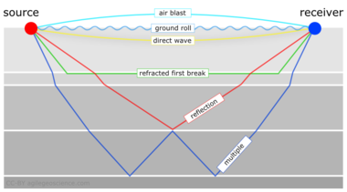
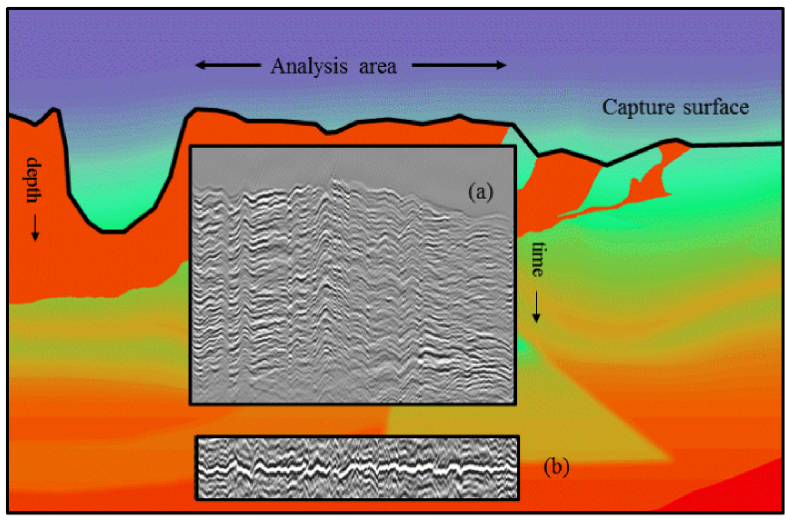
It isn't immediately intuitive why illuminating shallow targets can be troublesome, but with land seismic surveying in particular, first breaks and near surface refractions clobber shallow reflecting events. In the CMP domain, these are linear signals, used for determining statics, and are discarded by muting them out before migration. Reflections that arrive later than the direct wave and first refractions don't get muted out. But if these reflections arrive later than the air blast noise or ground roll noise — pervasive at near offsets — they get caught up in noise too. This region of the gather isn't muted like the top mute, otherwise you'd remove the data at near offsets. Instead, the gathers are attacked with algorithms to eliminate the noise. The extent of each hyperbola that passes through to migration is what we call the range of useful offsets.

The deepest reflections have plenty of useful offsets. However if we wanted to do adequate imaging somewhere between the first two reflections, for instance, then we need to make sure that we record redundant ray paths over this smaller range as well. We sometimes call this aperture; the shallow reflection is restricted in the number of offsets that it can be illuminated with, the deeper reflections can tolerate an aperture that is more open. In this image, I'm modelling the case of 60 geophones spanning 3000 metres, spaced evenly at 100 metres apart. This layout suggests merely 4 or 5 ray paths will hit the uppermost reflection, the shortest ray paths at small offsets. Also, there is usually no geophone directly on top of the source location to record a vertical ray path at zero offset. The deepest reflections however, should have plenty of fold, as long as NMO stretch, geometric spreading, and noise levels were good.

The problem with determining the range of useful offsets by way of a model is, not only does it require a velocity profile, which is easily attained from a sonic log, VSP, or velocity analysis, but it also requires an estimation of the the speed, intensity, and duration of the near surface events to be muted. Parameters that depend largely on the nature of the source and the local ground conditions, which vary from place to place, and from one season to the next.

In a future post, we'll apply this notion of useful offsets to build a pattern for shooting a 3D.

---

Click here for details on how I created this figure using the IPython Notebook. If you don't have it, IPython is easy to install. The easiest way is to install all of scientific Python, or use Canopy or Anaconda.

This post was inspired in part by Norm Cooper's 2004 article, A world of reality: Designing 3D seismic programs for signal, noise, and prestack time-migration. The Leading Edge23 (10), 1007-1014.DOI: 10.1190/1.1813357

Update on 2014-12-17 13:04 by Matt Hall
Don't miss the next installment — Laying out a seismic survey — with more IPython goodness!

Neglected near-surface workhorses

Yesterday afternoon, I attended a talk at Dalhousie by Peter Cary who has begun the CSEG distinguished lecture tour series. Peter's work is well known in the seismic processing world, and he's now spreading his insights to the broader geoscience community. This was only his fourth stop out of 26 on the tour, so there's plenty of time to catch it.

Three steps of seismic processing

In the head-spinning jargon of seismic processing, if you're lost, it's maybe not be your fault. Sometimes it might even seem like you're going in circles.

Ask the vendor or processing specialist first to keep it simple, and second to tell you in which of the three processing stages you are in. Seismic data processing has steps:

• Attenuate all types of noise.
• Remove the effects of the near surface.
• Migration, sometimes called imaging.

If time migration is the workshorse of seismic processing, and if is f–k filtering (or f–anything filtering) is the workhorse of noise attenuation, then surface consistent deconvolution is the workhorse of the near surface. These topics aren't as sexy or as new as FWI or compressed sensing, but Peter has been questioning the basics of surface-consistent scaling, and the approximations we make when processing land seismic data. 

The ambiguity of phase and travel-time corrections

To the processor, removing the effects of the near surface means making things flat in the CMP domain. It turns out you can do this with travel time corrections (static shifts), you can do this with phase corrections, or you can do it with both.

A simple synthetic example showing (a) a gather with surface-consistent statics and phase variations; (b) the same gather after surface-consistent residual statics correction, and (c) after simultaneous surface-consistent statics and phase correcition. Image © Cary & Nagarajappa and CSEG.

It's troubling that there is more than one way to achieve flatness. Peter's advice is to use shot stacks and receiver stacks to compare the efficacy of static corrections. They eliminate doubt about whether surface consistent scaling is working, and are a better QC tool than other data domains.

Deeper than shallow

It may sound trivial, but the hardest part about using seismic waves for imaging is that they have to travel down and back up through the near surface on their path to the target. It might seem counter-intuitive, but the geometric configurations that work well for the deep earth are not well suited to the shallow earth, and how we might correct for it. I can imagine that two surveys could be useful, one for the target and one for characterizing the shallow that gets in the way of the target, but seismic experiments are already expensive enough when there is only target to be concerned with.

Still, the near surface is something we can't avoid. Much like astronomers using ground-based telescopes shooting for the stars, seismic processors too have to get the noisy stuff that is sitting closest to the detectors out of the way.

Another 52 Things hits the shelves

The new book is out today: 52 Things You Should Know About Palaeontology. Having been up for pre-order in the US, it is now shipping. The book will appear in Amazons globally in the next 24 hours or so, perhaps a bit longer for Canada.

I'm very proud of this volume. It shows that 52 Things has legs, and the quality is as high as ever. Euan Clarkson knows a thing or two about fossils and about books, and here's what he thought of it: 

This is sheer delight for the reader, with a great range of short but fascinating articles; serious science but often funny. Altogether brilliant!

Each purchase benefits The Micropalaeontological Society's Educational Trust, a UK charity, for the furthering of postgraduate education in microfossils. You should probably go and buy it now before it runs out. Go on, I'll wait here...

1000 years of fossil obsession

So what's in the book? There's too much variety to describe. Dinosaurs, plants, foraminifera, arthropods — they're all in there. There's a geographical index, as before, and also a chronostratigraphic one. The geography shows some distinct clustering, that partly reflects the emphasis on the science of applied fossil-gazing: biostratigraphy. 

The book has 48 authors, a new record for these collections. It's an honour to work with each of them — their passion, commitment, and professionalism positively shines from the pages. Geologists and fossil nuts alike will recognize many of the names, though some will, I hope, be new to you. As a group, these scientists represent  1000 years of experience!

---

Amazingly, and completely by chance, it is one year to the day since we announced 52 Things You Should Know About Geology. Sales of that book benefit The AAPG Foundation, so today I am delighted to be sending a cheque for $1280 to them in Tulsa. Thank you to everyone who bought a copy, and of course to the authors of that book for making it happen.

R is for Resolution

Resolution is becoming a catch-all term for various aspects of the quality of a digital signal, whether it's a photograph, a sound recording, or a seismic volume.

I got thinking about this on seeing an ad in AAPG Explorer magazine, announcing an 'ultra-high-resolution' 3D in the Gulf of Mexico (right), aimed at site-survey and geohazard detection. There's a nice image of the 3D, but the only evidence offered for the 'ultra-high-res' claim is the sample interval in space and time (3 m × 6 m bins and 0.25 ms sampling). This is analogous to the obsession with megapixels in digital photography, but it is only one of several ways to look at resolution. The effect of increasing the sample interval of some digital images is shown in the second column here, compared to 200 × 200 pixels originals (click to zoom):

Another aspect of resolution is spatial bandwidth, which gets at resolving power, perhaps analogous to focus for a photographer. If the range of frequencies is too narrow, then broadband features like edges cannot be represented. We can simulate poor frequency content by bandpassing the data, for example smoothing it with a Gaussian filter (column 3).

Yet another way to think about resolution is precision (column 4). Indeed, when audiophiles talk about resolution, they are talking about bit depth. We usually record seismic with 32 bits per sample, which allows us to discriminate between a large number of values — but we often view seismic with only 6 or 8 bits of precision. In the examples here, we're looking at 2 bits. Fewer bits means we can't tell the difference between some values, especially as it usually results in clipping.

If it comes down to our ability to tell events (or objects, or values) apart, then another factor enters the fray: signal-to-noise ratio. Too much noise (column 5) impairs our ability to resolve detail and discriminate between things, and to measure the true value of, say, amplitude. So while we don't normally talk about the noise level as a resolution issue, it is one. And it may have the most variety: in seismic acquisition we suffer from thermal noise, line noise, wind and helicopters, coherent noise, and so on.

I can only think of one more impairment to the signals we collect, and it may be the most troubling: the total duration or extent of the observation (column 6). How much information can you afford to gather? Uncertainty resulting from a small window is the basis of the game Name That Tune. If the scale of observation is not appropriate to the scale we're interested in, we risk a kind of interpretation 'gap' — related to a concept we've touched on before — and it's why geologists' brains need to be helicoptery. A small 3D is harder to interpret than a large one. 

The final consideration is not a signal effect at all. It has to do with the nature of the target itself. Notice how tolerant the brick wall image is to the various impairments (especially if you know what it is), and how intolerant the photomicrograph is. In the astronomical image, the galaxy is tolerant; the stars are not. Notice too that trying to 'resolve' the galaxy (into a point, say) would be a mistake: it is inherently low-resolution. Indeed, its fuzziness is one of its salient features.

Have I missed anything? Are there other ways in which the recorded signal can suffer and targets can be confused or otherwise unresolved? How does illumination fit in here, or spectral bandwidth? What do you mean when you talk about resolution?

---

This post is an exceprt from my talk at SEG, which you can read about in this blog post. You can even listen to it if you're really bored. The images were generated by one of my IPython Notebooks that I point to in the talk, specifically images.ipynb. 

Astute readers with potent memories will have noticed that we have skipped Q in our A to Z. I just cannot seem to finish my post about Q, but I will!

The Safe Band ad is copyright of NCS SubSea. This low-res snippet qualifies as fair use for comment.

All the time freaks

Thursday was our last day at the SEG Annual Meeting. Evan and I took in the Recent developments in time-frequency analysis workshop, organized by Mirko van der Baan, Sergey Fomel, and Jean-Baptiste Tary (Vienna). The workshop came out of an excellent paper I reviewed this summer, which was published online a couple of weeks ago:

Tary, JB, RH Herrera, J Han, and M van der Baan (2014), Spectral estimation—What is new? What is next?, Rev. Geophys. 52. doi:10.1002/2014RG000461.

The paper compares the results of several time–frequency transforms on a suite of 'benchmark' signals. The idea of the workshop was to invite further investigation or other transforms. The organizers did a nice job of inviting contributors with diverse interests and backgrounds. The following people gave talks, several of them sharing their code (*):

• John Castagna (Lumina) with a review of the applications of spectral decomposition for seismic analysis.
• Steven Lin (NCU, Taiwan) on empirical methods and the Hilbert–Huang transform.
• Hau-Tieng Wu (Toronto) on the application of transforms to monitoring respiratory patterns in animals.*
• Marcílio Matos (SISMO) gave an entertaining, talk about various aspects of the problem.
• Haizhou Yang (Standford) on synchrosqueezing transforms applied to problems in anatomy.*
• Sergey Fomel (UT Austin) on Prony's method... and how things don't always work out.*
• Me, talking about the fidelity of time–frequency transforms, and some 'unsolved problems' (for me).*
• Mirko van der Baan (Alberta) on the results from the Tary et al. paper.

Some interesting discussion came up in the two or three unstructured parts of the session, organized as mini-panel discussions with groups of authors. Indeed, it felt like the session could have lasted longer, because I don't think we got very close to resolving anything. Some of the points I took away from the discussion:

• My observation: there is no existing survey of the performance of spectral decomposition (or AVO) — these would be great risking tools.
• Castagna's assertion: there is no model that predicts the low-frequency 'shadow' effect (confusingly it's a bright thing, not a shadow).
• There is no agreement on whether the so-called 'Gabor limit' of time–frequency localization is a lower-bound on spectral decomposition. I will write more about this in the coming weeks.
• Should we even be attempting to use reassignment, or other 'sharpening' tools, on broadband signals? To put it another way: does instantaneous frequency mean anything in seismic signals?
• What statistical measures might help us understand the amount of reassignment, or the precision of time–frequency decompositions in general?

The fidelity of time–frequency transforms

My own talk was one of the hardest I've ever done, mainly because I don't think about these problems very often. I'm not much of a mathematician, so when I do think about them, I tend to have more questions than insights, so I made my talk into a series of questions for the audience. I'm not sure I got much closer to any answers, but I have a better idea of my questions now... which is a kind of progress I suppose.

Here's my talk (latest slides — GitHub repo). Comments and feedback are, as always, welcome.

Big imaging, little imaging, and telescopes

I caught three lovely talks at the special session yesterday afternoon, Recent Advances and the Road Ahead. Here are my notes...

The neglected workhorse

If you were to count up all the presentations at this convention on seismic migration, only 6% of them are on time migration. Even though it is the workhorse of seismic data processing, it is the most neglected topic in migration. It's old technology, it's a commodity. Who needs to do research on time migration anymore? Sergey does.

Speaking as an academic, Fomel said, "we are used to the idea that most of our ideas are ignored by industry," even though many transformative ideas in the industry can be traced back to academics. He noted that it takes at least 5 years to get traction, and the 5 years are up for his time migration ideas, "and I'm starting to lose hope". Here's five things you probably didn't know about time migration:

• Time migration does not need travel times.
• Time migration does not need velocity analysis.
• Single offsets can be used to determine velocities.
• Time migration does need approximations, but the approximation can be made increasingly accurate.
• Time migration distorts images, but the distortion can be removed with regularized inversion.

It was joy to listen to Sergey describe these observations through what he called beautiful equations: "the beautiful part about this equation is that it has no parameters", or "the beauty of this equation is that is does not contain velocity", an so on. Mad respect.

Seismic adaptive optics

Alongside seismic multiples, poor illumination, and bandwidth limitations, John Etgen (BP) submitted that, in complex overburden, velocity is the number one problem for seismic imaging. Correct velocity model equals acceptable image. His (perhaps controversial) point was that when velocities are complex, multiples, no matter how severe, are second order thorns in the side of the seismic imager. "It's the thing that's killing us, and that's the frontier." He also posited that full waveform inversion may not save us after all, and image gather analysis looks even less promising.

While FWI looks to catch the wavefield and look at it in the space of the data, migration looks to catch the wavefield and look at it at the image point itself. He elegantly explained these two paradigms, and suggested that both may be flawed.

John urged, "We need things other than what we are working on", and shared his insights from another field. In ground-based optical astronomy, for example, when the image of a star is be distorted by turbulence in our atmosphere, astromoners numerically warp the curvature of the lens to correct for rapid variations in phase of the incoming wavefront. The lenses we use for seismic focusing, velocities, can be tweaked just the same by looking at the wavefield part of the way through its propagation. He quoted Jon Claerbout:

If you want to understand how a horse runs, you gotta run along with it.

Big imaging, little imaging, and combination of the two

There's a number of ways one could summarize what petroleum seismologists do. But hearing (CGG researcher) Sam Gray's talk yesterday was a bit of an awakening. His talk was a remark on the notion of big imaging vs little imaging, and the need for convergence.

Big imaging is the structural stuff. Structural migration, stratigraphic imaging, wide-azimuth acquisition, and so on. It includes the hardware and compute innovations of broadband, blended sources, deblending processing, anisotropic imaging, and the beginnings of viscoacoustic reverse-time migration. 

Little imaging is inversion. It's reservoir characterization. It's AVO and beyond. Azimuthal velocities (fast and slow directions) hint at fracture orientations, azimuthal amplitudes hint even more subtly at fracture compliance.

Big imaging is hard because it's computationally expensive, and velocities are unknown. Little imaging is hard because features like fractures, faults and pores are at the centimetre scale, but on land we lay out inlines and crossline hundreds of metres apart, and use signals that carry only a few bits of information from an area the size of a football field.

What we've been doing with imaging is what he called a separated workflow. We use gathers to make big images. We use gathers to make rock properties, but seldom do they meet. How often have you tested to see if the rock properties the little are explain the wiggles in the big? Our work needs to be such a cycle, if we want our relevance and impact to improve.

The figures are copyright of the authors of SEG, and used in accordance with SEG's permission guidelines.

October linkfest

The linkfest has come early this month, to accommodate the blogging blitz that always accompanies the SEG Annual Meeting. If you're looking forward to hearing all about it, you can make sure you don't miss a thing by getting our posts in your email inbox. Guaranteed no spam, only bacn. If you're reading this on the website, just use the box on the right →

---

Open geoscience goodness

I've been alerted to a few new things in the open geoscience category in the last few days:

• Dave Hale released his cool-looking fault detection code
• Wayne Mogg released some OpendTect plugins for AVO, filtering, and time-frequency decomposition
• Joel Gehman and others at U of A and McGill have built WellWiki, a wiki... for wells!
• Jon Claerbout, Stanford legend, has released his latest book with Sergey Formel, Austin legend: Geophysical Image Estimation by Example. As you'd expect, it's brilliant, and better still: the code is available. Amazing resource.

And there's one more resource I will mention, but it's not free as in speech, only free as in beer — Petroacoustics: A Tool for Applied Seismics, by Patrick Rasolofosaon and Bernard Zinszner. So it's nice because you can read it, but not that useful because the terms of use are quite stringent. Hat tip to Chris Liner.

So what's the diff if things are truly open or not? Well, here's an example of the good things that happen with open science: near-real-time post-publication peer review and rapid research: How massive was Dreadnoughtus?

Technology and geoscience

Open data sharing has great potential in earthquake sensing, as there are many more people with smartphones than there are seismometers. The USGS shake map (right) is of course completely perceptual, but builds in real time. And Jawbone, makers of the UP activity tracker, were able to sense sleep interruption (in their proprietary data): the first passive human-digital sensors?

We love all things at the intersection of the web and computation... so Wolfram Alpha's new "Tweet a program" bot is pretty cool. I asked it:

GeoListPlot[GeoEntities[=[Atlantic Ocean], "Volcano"]]

And I got back a map!

This might be the coolest piece of image processing I've ever seen. Recovering sound from silent video images:

Actually, these time-frequency decompositions [PDF] of frack jobs are just as cool (Tary et al., 2014, Journal of Geophysical Research: Solid Earth 119 (2), 1295-1315). These deserve a post of their own some time.

It turns out we can recover signals from all sorts of unexpected places. There were hardly any seismic sensors around when Krakatoa exploded in 1883. But there were plenty of barometers, and those recorded the pressure wave as it circled the earth — four times! Here's an animation from the event.

It's hard to keep up with all the footage from volcanic eruptions lately. But this one has an acoustic angle: watch for the shockwave and the resulting spontaneous condensation in the air. Nonlinear waves are fascinating because the wave equation and other things we take for granted, like the superposition principle and the speed of sound, no longer apply.

Discussion and collaboration

Our community has a way to go before we ask questions and help each other as readily as, say, programmers do, but there's enough activity out there to give hope. My recent posts (one and two) about data (mis)management sparked a great discussion both here on the blog and on LinkedIn. There was also some epic discussion — well, an argument — about the Lusi post, as it transpired that the story was more complicated that I originally suggested (it always is!). Anyway, it's the first debate I've seen on the web about a sonic log. And there continues to be promising engagement on the Earth Science Stack Exchange. It needs more applied science questions, and really just more people. Maybe you have a question to ask...?

Géophysiciens avec des ordinateurs

Don't forget there's the hackathon next weekend! If you're in Denver, free come along and soak up the geeky rays. If you're around on the afternoon of Sunday 26 October, then drop by for the demos and prizes, and a local brew, at about 4 pm. It's all happening at Thrive, 1835 Blake Street, a few blocks north of the convention centre. We'll all be heading to the SEG Icebreaker right afterwards. It's free, and the doors will be open.

Great geophysicists #12: Gauss

Carl Friedrich Gauss was born on 30 April 1777 in Braunschweig (Brunswick), and died at the age of 77 on 23 February 1855 in Göttingen. He was a mathematician, you've probably heard of him; he even has his own Linnean handle: Princeps mathematicorum, or Prince of mathematicians (I assume it's the royal kind, not the Purple Rain kind — ba dum tss).

Gauss's parents were poor, working class folk. I wonder what they made of their child prodigy, who allegedly once stunned his teachers by summing the integers up to 100 in seconds? At about 16, he was quite a clever-clogs, rediscovering Bode's law, the binomial theorem, and the prime number theorem. Ridiculous.

His only imperfection was that he was too much of a perfectionist. His motto was pauca sed matura, meaning "few, but ripe". It's understandable how someone so bright might not feel much need to share his work, but historian Eric Temple Bell reckoned that if Gauss had published his work regularly, he would have advanced mathematics by fifty years.

He was only 6 when Euler died, but surely knew his work. Euler is the only other person who made comparably broad contributions to what we now call the exploration geophysics toolbox, and applied physics in general. Here are a few: 

• He proved the fundamental theorems of algebra and arithmetic. No big deal.
• He formulated the Gaussian function — which of course crops up everywhere, especially in geostatistics. The Ricker wavelet is a pulse with frequencies distributed in a Gaussian.
• The gauss is the cgs unit of magnetic flux density, thanks to his work on the flux theorem, one of Maxwell's equations.
• He discovered the Cauchy integral theorem for contour integrals but did not publish it.
• The 'second' or 'total' curvature — a coordinate-system-independent measure of spatial curvedness — is named after him.
• He made discoveries in non-Euclidean geometry, but did not publish them.

Excitingly, Gauss is the first great geophysicist we've covered in this series to have been photographed (right). Unfortunately, he was already dead. But what an amazing thing, to peer back through time almost 160 years.

Next time: Augustin-Jean Fresnel, a pioneer of wave theory.

The hackathon is coming

The Geophysics Hackathon is one month away! Signing up is not mandatory — you can show up on the day if you like — but it does help with the planning. It's 100% free, and I guarantee you'll enjoy yourself. You'll also learn tons about geophysics and about building software. Deets: Thrive, Denver, 8 am, 25–26 October. Bring a laptop.

Need more? Here's all the info you could ask for. Even more? Ask by email or in the comments. 

Send your project ideas

The theme this year is RESOLUTION. Participants are encouraged to post projects to hackathon.io ahead of time — especially if you want to recruit others to help. And even if you're not coming to the event, we'd love to hear your project ideas. Here are some of the proto-ideas we have so far: 

• Compute likely spatial and temporal resolution from some basic acquisition info: source, design, etc.
• Do the same but from information from the stack: trace spacing, apparent bandwidth, etc.
• Find and connect literature about seismic and log resolution using online bibliographic data.
• What does the seismic spectrum look like, given STFT limitations, or Gabor uncertainty?

If you have a bright idea, get in touch by email or in the comments. We'd love to hear from you.

Thank you to our sponsors

Three forward-thinking companies have joined us in making the hackathon as much a geophysics party as well as a scientific workshop (a real workshop). I think this industry may have trained us to take event sponsorship for granted, but it's easy to throw $5000 at the Marriott for Yet Another Coffee Break. Handing over money to a random little company in Nova Scotia to buy coffee, tacos, and cool swag for hungry geophysicists and programmers takes real guts! 

Please take a minute to check out our sponsors and reward them for supporting innovation in our community. 

Students: we are offering $250 bursaries to anyone looking for help with travel or accommodation. Just drop me a line with a project idea. If you know a student that might enjoy the event, please forwadrd this to them.

The road to Modelr: my EuroSciPy poster

At EuroSciPy recently, I gave a poster-ized version of the talk I did at SciPy. Unlike most of the other presentations at EuroSciPy, my poster didn't cover a lot of the science (which is well understood), or the code (which is esoteric).

Instead it focused on the advantages of spreading software via web applications, rather than only via source code, and on the challenges that we overcame — well, that we're still overcoming — to get our Modelr tool out there. I wanted other programmer-scientists to think about running some of their code as a web app for others to enjoy, but to be aware of the effort involved in doing this.

I've written before about my dislike of posters, though I'm told they are an important component at, say, the AGU Fall Meeting. I admit I do quite like the process of making them, and — on advice from Colin Purrington's useful page — I left a space on the poster for people to write comments or leave sticky notes. As a result, I heard about Docker, a lead I'll certainly follow up,

What's new in modelr

This wasn't part of the poster, but I might as well take the chance to let you know what we've updated recently:

• You can now add noise to models by specifying the signal:noise.
• Instead of automatic scaling, you can choose your own gain.
• The app now returns the elastic moduli of the rocks in the model.
• You can choose a spatial cross-section view or a space–offset–frequency view.

All of these features are now available to subscribers for only $9/month. Amazing value :)

Figshare

I've stored my poster on Figshare, a data storage site and part of Macmillan's Digital Science effort. What I love about Figshare, apart from the convenience of cloud-based storage and easy access for others, is that every item gets a digital object identifier or DOI. You've probably seen these on journal articles. They're a bit like other persistent and unique IDs for publications, such as ISBNs for books, but the idea is to provide more interactivity by making it easily linkable: you can get to any object with a DOI by prepending it with "http://dx.doi.org/".

Reference

Hall, M (2014). The road to modelr: building a commercial web app on an open source foundation. EuroSciPy, Cambridge, UK, August 29–30, 2014. Poster presentation. DOI:10.6084/m9.figshare.1151653