The deep time clock

Check out this video by a Finnish Lego engineer on the Brick Experiment Channel (BEC):

This brilliant, absurd machine — which fits easily on a coffee table — made me think about geological time.

Representing deep time is a classic teaching problem in geoscience. Most of them are variants of “Imagine the earth’s history compressed into 24 hours” and use a linear scale. It’s amazing how even the Cretaceous is only 25 minutes long, and humans arrived a few seconds ago. These memorable and effective demos have been blowing people’s minds for years.

Clocks with v e r y s l o w hands

I think an even nicer metaphor is the clock. Although non-linear, it’s instantly familiar, even if its inner workings of cogs and gears are not. We all understand how the hands move with different periods (especially if you’ve ever had a dull job). So this image (right) from the video is, I think, a nice lead-in to what ends up being a mind-exploding depiction of deep time, beyond anything you can do with a linear analogy.

Indeed, if the googol-gear-machine viking minifigure rotation was a day, the Cretaceous essentially doesn’t exist. Nothing does, it’s just 24 hours of protons decaying.

After a couple of giant gears, the engineer adds this chain of gears (below). Once attached to the rest of the machine, these things — the first 10 of them anyway — are essentially the hands on a geological clock.

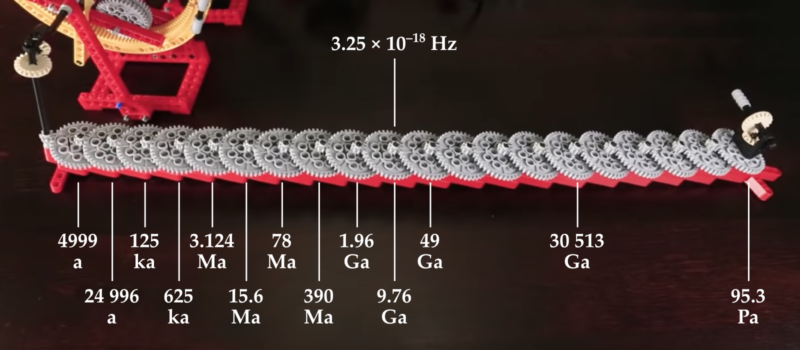
The first hand on this clock, so to speak, turns once every 4999 years. This is not a bad unit of measure if you’re looking at earth surface processes. Then each new gear multiplies by a factor of 40/8, so the next one is 25 ka, and the next 125 ka — around the domain of Milankovich cycles. Then things start getting really geological. The 5th clock hand does one rotation every 3.1 million years, then the 6th is 15.6 Ma. Unfortunately it quickly gets out of hand: the 10th has only turned once since the start of the universe, and after that they are all basically useless for thinking about anything but cosmological timelines. The last one here turns once every 95 petayears.

Remarkably, the BEC machine is still just getting started here. 95 Pa is nothing compared to the last wheel, which would require more energy than exists in the universe to turn. Think about that.

I want one of these

Apparently the BEC machine was inspired by a Daniel de Bruin creation:

Each wheel here is a 100:10 reduction. You’d only need the first 20 of them to have the last one do one single revolution since the birth of the solar system!

If someone would like to build such a geological clock for me, I’ll pay a sub-googol amount of money for it. Bonus points if it fits in a wristwatch.

The hot rock hack happened

I was excited about the World Geothermal Congress this year. (You remember conferences — big, expensive, tiring lecture-marathons that scientists used to go to. But sometimes they were fun.)

Until this year, the WGC has only happened every 5 years and we missed the last one because it was in Australia… and the 2023 edition (it’s moving to a 3-year cycle) will be in China. So this year’s event, just a stone’s throw away in Iceland, was hotly anticipated.

And it still is, because now it will be next May. And we’ll be doing a hackathon there! You should come, get it in your calendar: 27 and 28 May 2021.

Meanwhile, this year… we moved our planned hackathon online. For the record, here’s what happened at the first Geothermal Hackathon.

Logistics: Timezones are tricky

There’s no doubt, the biggest challenge was the rotation of the earth (though admittedly it has other benefits). I believe the safest way to communicate times to a global audience is UTC, so I’ll stick to that here. It’s not ideal for anyone (except Iceland, appropriately enough in this case) but it reduces errors. We started at 0600 UTC and went until about 2100 UTC each day; about 15 hours of fun. I did check in briefly at 0000 UTC on each morning (my evening), in case anyone from New Zealand showed up, but no-one did.

Rob Leckenby and Martin Bentley, both in the UTC+2 zone, handled the early morning hosting, with me, Evan and Diego showing up a few hours later (we’re all in Canada, UTC–a few). This worked pretty well even though, as usual, the hackers were all perfectly happy and mostly self-sufficient whether we were there or not.

Technology-wise, we met up on Zoom, which was good for the start and the end of the day, and also for getting the attention of others in between (many people left the audio open, one ear to the door, so to speak.) Alongside Zoom we used the Software Underground’s Slack. As well as the #geothermal channel, each project had a channel — listed below — which meant that each project could have a separate video meetup at any time, as well as text-based chat and code-sharing. It was a good combination.

Let’s have a look at the hacks.

---

Six projects

An awesome list for geothermal — #geothermal-awesome — Thomas Martin (Colorado School of Mines), with some input from me and others, made a great start on an ‘awesome list’ document for geothermal, with a machine learning amphasis. He lists papers, tools, and open data. You can read (or contribute to!) the document here.

Collaboration tools for geothermal teams — #geothermal-collaboration-tools — Alex Hobé (Uppsala) and Valentin Métraux (GEO2X), with input from Martin Bentley and others, had a clear vision for the event: he wanted to map out the flow of data and interpretations between professionals in a geothermal project. I’ve seen similar projects get nowhere near as far in 2 months as Alex got in 2 days. The team used Holoviews and NetworkX to make some nice graphics.

GEOPHIRES web app — #geothermal-geophires — Marko Gauk (SeisWare) wanted to get into web apps at the event, and he succeeded! He built a web-based form for submitting jobs to a server running GEOPHIRES v2, a ‘full field’ geothermal project modeling tool. You can check out his app here.

Geothermal Natural Language Processing — #geothermal-nlp — Mohammad ‘Jabs’ Aljubran (Stanford), Friso (Denver), along with Rob and me, did some playing with the Stanford geothermal bibliographic database. Jabs and Friso got a nice paper recommendation engine working, while Rob and I managed to do automatic geolocation on the articles — and Jabs turned this into some great maps. Repo is here. Coming soon: a web app.

Experiments with porepy — #geothermal-porepy — Luisa Zuluaga, Daniel Coronel, and Sam got together to see what they could do with porepy, a porous media simulation tool, especially aimed at modeling fractured and deformable rocks.

Radiothermic map of Nova Scotia — #geothermal-radiothermic — Evan Bianco downloaded some open data for Nova Scotia, Canada, to see if he could implement this workflow from Beamish and Busby. But the data turned out to be unscaled (among other things), and therefore probably impossible to use for quantitative purposes. At least he made progress on a nice map.

All in all it was a fun couple of days. You can’t beat a hackathon for leaving behind emails and to-do lists for a day

Stratigraphic interpretation

Over the weekend, Lisa Stright posted a question on the Software Underground’s Slack:

“[… W]hat are you favorite seismic attributes for analyzing subtle stratigraphic changes in vertical sections (not time or strata slices)? I’m trying to quantitatively analyze sedimentological information from seismic data and am curious about either best practices and/or useful approaches in reservoir geophysics.”

I really like questions like this, because they tend to bring out a lot of useful tricks and ideas from the community. However, my own response turned into a bit of a wall of text, so I thought I’d unpack it a bit here, with some links and detail.

I’ll start with the general advice for any reservoir seismic interpretation:

1. Before trying any interpretation that relies on reflector patterns, it’s crucial to make sure the phase is good. There are two really good papers to read on phase determination: Roden & Sepulveda (1999) and Perz, Sacchi and O’Byrne (2004). I summarized this in the SubSurfWiki article on phase determination. (Note to self: it would be fun to write a tool to semi-automate some of these tests.)

2. Always use at least 16-bit, unfiltered data for attributes. If you’re having data processed, it’s important to ask for unfiltered data, because in my experience most processors just can’t help themselves.

3. If using marine data, it's imperative that you know where to expect multiples because they can create convincing pinch out etc. Make integer multiples of the seafloor to help predict — and there are lots of other horizons you could make.

4. You need to know the tuning thickness for the interval of interest. You can compute it with the uppermost frequency, \(f_\mathrm{max}\) (the frequency when the normalized power hites –20 dB down) and velocity \(v\) as \(v / 4f_\mathrm{max}\) (n.b. spatial resolution is \(v / 2f_\mathrm{max}\)). Amplitudes that you can interpret as tuning effect might help you spot thickness variations in thin beds near and below seismic resolution.

As for the attributes, I've never got on with fancy 'pattern' attributes like parallelism, although it is different from anything else. Plenty of experienced interpreters mention cosine of phase too, but again I don’t recall having used it on the battlefield; perhaps I’m missing out, or maybe my data’s just never been suitable.

Instead, here are the ones I tend to go for:

1. Integrated trace is the most under-appreciated attribute, in my opinion. It is sometimes called relative acoustic impedance and is incredibly cheap to compute.

2. Semblance is a genuinely different view of your data, at least in stratal slices. (I realize now that Lisa explicitly said she wasn’t interested in stratal horizontal attributes, but I‘ll leave it in for completeness Same for the next one…)

3. Spectral decomposition is a good tool if done carefully, again in stratal slices. Stick to the band of your data though.

By the way, before doing anything important with attributes, read everything you can by Art Barnes, starting with Too many seismic attributes? (Barnes 2006). TL;DR — he says there are only 10 you need to know about.

Advice from other interpreters

Art Barnes isn’t the only one with good advice to offer!

In the same Slack thread, Steve Purves (who wrote a nice Geophysical Tutorial about phase) mentioned the awesome PyLops tutorial on coloured inversion (PyLops is a linear operator package from Equinor). And Rob G also pointed out the merits of inversion for stratigraphic interpretation. (With the added bonus that you don’t need absolute impedance from it, so a lot of the usual inversion challenges, like low-frequency models, aren’t quite as critical).

Rob G also had this awesome advice:

“I would also have a look at the amplitude-frequency spectrum of your seismic data compare it to the spectra of your well acoustic impedance logs (in your AOI). Then consider doing some spectral shaping to enhance the higher frequencies in the seismic to match the well logs (spectral blueing). This should allow you to see more details, however you have to be very careful to ensure you are not over boosting the higher frequencies which contain more noise than signal.”

Finally, Doug McClymont, who I know from several events in the UK to be a wise geophysicist, underscored the usefulness of both the ‘instantaneous phase of the peak envelope’ and the ‘phase rotation with the highest amplitude’ methods, especially when well ties are prone to unresolvable time shift residuals. Great advice.

As the Software Underground continues to evolve, these are the conversations that keep it awesome.

---

References

• Barnes, A (2006). Too many seismic attributes? CESG Recorder 31 (3). Available online.

• Perz, M, M Sacchi and A O'Byrne (2004). Instantaneous phase and the detection of lateral wavelet stability. The Leading Edge 23 (7), 639–643. DOI 10.1190/1.1776731.

• Purves, S (2014). Geophysical Tutorial: Phase and the Hilbert transform. The Leading Edge 33, p 1164–1166. DOI 10.1190/tle33101164.1

• Roden, R and H Sepulveda (1999). The significance of phase to the interpreter; practical guidelines for phase analysis The Leading Edge 18 (7), p. 774–777. DOI 10.1190/1.1438375