How good is what?

Geology is a descriptive science, which is to say, geologists are label-makers. We record observations by assigning labels to data. Labels can either be numbers or they can be words. As such, of the numerous tasks that machine learning is fit for attacking, supervised classification problems are perhaps the most accessible – the most intuitive – for geoscientists. Take data that already has labels. Build a model that learns the relationships between the data and labels. Use that model to make labels for new data. The concept is the same whether a geologist or an algorithm is doing it, and in both cases we want to test how well our classifier is at doing its label-making.

2d_2class_classifier_left.png

Say we have a classifier that will tell us whether a given combination of rock properties is either a dolomite (purple) or a sandstone (orange). Our classifier could be a person named Sally, who has seen a lot of rocks, or it could be a statistical model trained on a lot of rocks (e.g. this one on the right). For the sake of illustration, say we only have two tools to measure our rocks – that will make visualizing things easier. Maybe we have the gamma-ray tool that measures natural radioactivity, and the density tool that measures bulk density. Give these two measurements to our classifier, and they return to you a label. 

How good is my classifier?

Once you've trained your classifier – you've done the machine learning and all that – you've got yourself an automatic label maker. But that's not even the best part. The best part is that we get to analyze our system and get a handle on how good we can expect our predictions to be. We do this by seeing if the classifier returns the correct labels for samples that it has never seen before, using a dataset for which we know the labels. This dataset is called validation data.

Using the validation data, we can generate a suite of statistical scores to tell us unambiguously how this particular classifier is performing. In scikit-learn, this information compiled into a so-called classification report, and it’s available to you with a few simple lines of code. It’s a window into the behaviour of the classifier that warrants deeper inquiry.

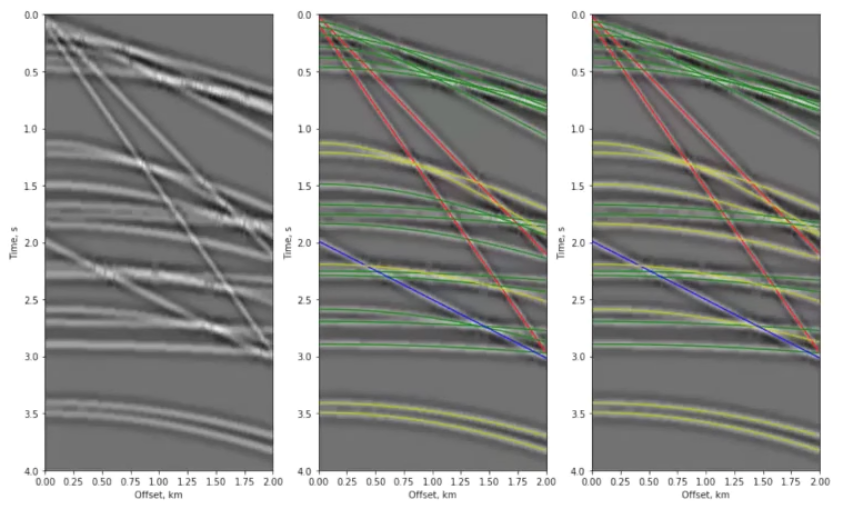
To describe various elements in a classification report, it will be helpful to refer to some validation data:

Our Two-class Classifier (left) has not seen the Validation Data (middle). We can calculate a classification report by Analyzing the intersection of the two (right).

Our Two-class Classifier (left) has not seen the Validation Data (middle). We can calculate a classification report by Analyzing the intersection of the two (right).

Accuracy is not enough

When people straight up ask about a model’s accuracy, it could be that they aren't thinking deeply enough about the performance of the classifier. Accuracy is a measure of the entire classifier. It tells us nothing about how well we are doing with one class compared to another, but there are other metrics that tell us this:

metric_definitions2.png

Support — how many instances there were of that label in the validation set.

Precision — the fraction of correct predictions for a given label. Also known as positive predictive value.

Recall — the proportion of the class that we correctly predicted. Also known as sensitivity.

F1 score — the harmonic mean of precision and recall. It's a combined metric for each class.

Accuracy – the total fraction of correct predictions for all classes. You can calculate this for each class, but it will be the same value for each of the class.   

DIY classification report

If you're like me and you find the grammar of true positives and false negatives confusing, it might help to to treat each class within the classifier as its own mini diagnostic test, and build up data for the classification report row by row. Then it's as simple as counting hits and misses from the validation data and computing some fractions. Inspired by this diagram on the Wikipedia page for the F1 score, I've given both text and pictorial versions of the equations:

dolomite_and_classifier_report_sheet.png

Have a go at filling in the scores for the two classes above. After that, fill in your answers into your own hand-drawn version of the empty table below. Notice that there is only a single score for accuracy for the entire classifier, and that there may be a richer story between the various other scores in the table. Do you want to optimize accuracy overall? Or perhaps you care about maximizing recall in one class above all else? What matters most to you? Should you penalize some mistakes stronger than others?

clf_report.png

When data sets get larger – by either increasing the number of samples, or increasing the dimensionality of the data – even though this scoring-by-hand technique becomes impractical, the implementation stays the same. In classification problems that have more than two classes we can add in a confusion matrix to our reporting, which is something that deserves a whole other post. 

Upon finishing logging a slab of core, if you were to ask Sally the stratigrapher, "How accurate are your facies?", she may dismiss your inquiry outright, or maybe point to some samples she's not completely confident in. Or she might tell you that she was extra diligent in the transition zones, or point to regions where this is very sandy sand, or this is very hydrothermally altered. Sadly, we in geoscience – emphasis on the science – seldom take the extra steps to test and report our own performance. But we totally could.

The ANSWERS. Upside Down. To two Decimal places.

The ANSWERS. Upside Down. To two Decimal places.

Weekend worship in Salt Lake City

The Salt Lake City hackathon — only the second we've done with a strong geology theme — is a thing of history, but you can still access the event page to check out who showed up and who did what. (This events page is a new thing we launched in time for this hackathon; it will serve as a public document of what happens at our events, in addition to being a platform for people to register, sponsor, and connect around our events.) 

In true seat-of-the-pants hackathon style we managed to set up an array of webcams and microphones to record the finale. The demos are the icing on the cake. Teams were selected at random and were given 4 minutes to wow the crowd. Here is the video, followed by a summary of what each team got up to... 


Unconformist.ai

Didi Ooi (University of Bristol), Karin Maria Eres Guardia (Shell), Alana Finlayson (UK OGA), Zoe Zhang (Chevron). The team used machine learning the automate the mapping of unconformities in subsurface data. One of the trickiest parts is building up a catalog of data-model pairs for GANs to train on. Instead of relying on thousand or hundreds of thousands of human-made seismic interpretations, the team generated training images by programmatically labelling pixels on synthetic data as being either above (white) or below (black) the unconformity. Project pageSlides.

unconformist.ai_preso

Outcrops Gee Whiz

Thomas Martin (soon Colorado School of Mines), Zane Jobe (Colorado School of Mines), Fabien Laugier (Chevron), and Ross Meyer (Colorado School of Mines). The team wrote some programs to evaluate facies variability along drone-derived digital outcrop models. They did this by processing UAV point cloud data in Python and classified different rock facies using using weather profiles, local cliff face morphology, and rock colour variations as attributes. This research will help in the development drone assisted 3D scanning to automate facies boundaries mapping and rock characterization. RepoSlides.

SLC_outcrop_geewhiz_blog.png

Jet Loggers

Eirik Larsen and Dimitrios Oikonomou (Earth Science Analytics), and Steve Purves (Euclidity). This team of European geoscientists, with their circadian clocks all out of whack, investigated if a language of stratigraphy can be extracted from the rock record and, if so, if it can be used as another tool for classifying rocks. They applied natural language processing (NLP) to an alphabetic encoding of well logs as a means to assist or augment the labour-intensive tasks of classifying stratigraphic units and picking tops. Slides.


SLC_NLP_jet_loggers.png
SLC_bookcliffs.png

Book Cliffs Bandits

Tom Creech (ExxonMobil) and Jesse Pisel (Wyoming State Geological Survey). The team started munging datasets in the Book Cliffs. Unfortunately, they really did not have the perfect, ready to go data, and by the time they pivoted to some workable open data from Alaska, their team name had already became a thing. The goal was build a tool to assist with lithology and stratigraphic correlation. They settled on change-point detection using Bayesian statistics, which they were using to build richer feature sets to test if it could produce more robust automatic stratigraphic interpretation. Repo, and presentation.


A channel runs through it

Nam Pham (UT Austin), Graham Brew (Dynamic Graphics), Nathan Suurmeyer (Shell). Because morphologically realistic 3D synthetic seismic data is scarce, this team wrote a Python program that can take seismic horizon interpretations from real data, then construct richer training data sets for building an AI that can automatically delineate geological entities in the subsurface. The pixels enclosed by any two horizons are labelled with ones, pixels outside this region are labelled with zeros. This work was in support of Nam's thesis research which is using the SegNet architecture, and aims to extract not only major channel boundaries in seismic data, but also the internal channel structure and variability – details that many seismic interpreters, armed even with state-of-the art attribute toolboxes, would be unable to resolve. Project page, and code.

GeoHacker

Malcolm Gall (UK OGA), Brendon Hall and Ben Lasscock (Enthought). Innovation happens when hackers have the ability to try things... but they also need data to try things out on. There is a massive shortage of geoscience datasets that have been staged and curated for machine learning research. Team Geohacker's project wasn't a project per se, but a platform aimed at the sharing, distribution, and long-term stewardship of geoscience data benchmarks. The subsurface realm is swimming with disparate data types across a dizzying range of length scales, and indeed community efforts may be the only way to prove machine-learning's usefulness and keep the hype in check. A place where we can take geoscience data, and put it online in a ready-to-use for for machine learning. It's not only about being open, online and accessible. Good datasets, like good software, need to be hosted by individuals, properly documented, enriched with tutorials and getting-started guides, not to mention properly funded. Website.

SLC_petrodict.png

Petrodict

Mark Mlella (Univ. Louisiana, Lafayette), Matthew Bauer (Anchutz Exploration), Charley Le (Shell), Thomas Nguyen (Devon). Petrodict is a machine-learning driven, cloud-based lithology prediction tool that takes petrophysics measurements (well logs) and gives back lithology. Users upload a triple combo log to the app, and the app returns that same log with with volumetric fractions for it's various lithologic or mineralogical constituents. For training, the team selected several dozen wells that had elemental capture spectroscopy (ECS) logs – a premium tool that is run only in a small fraction of wells – as well as triple combo measurements to build a model for predicting lithology. Repo.

Seismizor

George Hinkel, Vivek Patel, and Alex Waumann (all from University of Texas at Arlington). Earthquakes are hard. This team of computer science undergraduate students drove in from Texas to spend their weekend with all the other geo-enthusiasts. What problem in subsurface oil and gas did they identify as being important, interesting, and worthy of their relatively unvested attention? They took on the problem of induced seismicity. To test whether machine learning and analytics can be used to predict the likelihood that injected waste water from fracking will cause an earthquake like the ones that have been making news in Oklahoma. The majority of this team's time was spent doing what all good scientists do –understanding the physical system they were trying to investigate – unabashedly pulling a number of the more geomechanically inclined hackers from neighbouring teams and peppering them with questions. Induced seismicity is indeed a complex phenomenon, but George's realization that, "we massively overestimated the availability of data", struck a chord, I think, with the judges and the audience. Another systemic problem. The dynamic earth – incredible in its complexity and forces – coupled with the fascinating and politically charged technologies we use for drilling and fracking might be one of the hardest problems for machine learning to attack in the subsurface. 


AAPG next year is in San Antonio. If it runs, the hackathon will be 18–19 of May. Mark your calendar and stay tuned!

Woo yeah perfect: hacking in Salt Lake City

Thirty geoscientist-coders swarmed into Salt Lake City this past weekend to hack at Church & State, a co-working space in a converted church. There, we spent two days appealing to the almighty power of machine learning.

Nine teams worked on the usual rich variety of projects around the theme. Projects included AIs that pick unconformities, natural language processing to describe stratigraphy, and designing an open data platform in service of machine learning. 

I'll do a run-down of the projects soon, but if you can't wait until then for my summary, you can watch the demos here; the first presentation starts at the 38 minute mark of the video. And you can check out some pictures from the event:

Pictures can say a lot but a few simple words, chosen at the right time, can speak volumes too. Shortly before we launched the demos, we asked the participants to choose words that best described how they were feeling. Here's what we got:

word_cloud_menti_SLC.png

Each participant was able to submit three responses, and although we aren't able to tell who said what, we were able to scrape the data and look at each person's chosen triplet of words. A couple of noteworthy ones were: educated, naptimeinspired and the expressive woo, yeah, perfect. But my personal favorite, by far, has to be the combination of: dead, defeated, inspired.

The creative process can be a rollercoaster of emotions. It's not easy. It's not always comfortable. Things don't always work out. But that's entirely ok. Indeed, facing up to this discomfort, as individuals and as organizations, is a necesary step in the path to digital transformation.

Enough Zen! To all the participants who put in the hard work this weekend, and to our wonderful sponsors who brought all kinds of support, I thank you and I salute you.

sponsors.png

Fear and loathing in oil & gas

Sometimes you have to swallow your fear. This is one of those times.

The proliferation of 3D seismic in the 1980s was a major step forward for the petroleum industry. However, it took more than a decade for the 3D seismic method to become popular. During that decade, seismic equipment continued to evolve, particularly with the advent of telemetry recording systems that needed for doing 3D surveys offshore.

Things were never the same again. New businesses sprouted up to support it, and established service companies and tech companies exploded size and in order to keep up with the demand and all the new work.

Not so coincidently, another major shift happened in the late 1980s and early 1990s with the industry-wide shift to Sun workstations in order to cope with the crunching and rendering the overwhelming influx of all these digits. UNIX workstations with hilariously large cathode-ray tube monitors became commonplace. This industry helped make Sun and many other IT companies very wealthy, and once again everything was good. At least until Sun's picnic was trampled on by Linux workstations in the early 2000s, but that's another story...

I think the advent of 3D seismic is one of many examples of the upstream oil and gas industry thriving on technological change. 3D seismic changed everything, facilitating progress in the full sense of the word and we never looked back. As an early career geoscientist, I don't know what the world was like before 3D seismic, but I have interpreted 2D data and I know it's an awful experience — even on a computer.

Debilitating skepticism?

Today, in 2017, we find ourselves in the middle of the next major transformation. Like 3D seismic before it, machine learning will alter yesterday's landscape beyond all recognition. We've been through all of this before, but this time, for some reason it feels different. Many people are cautious, unconvinced about whether this next thing will live up to the hype. Other people are vibrating with excitement viewing the whole thing with rose-coloured glasses. Still others truly believe that it will fail — assertively rejecting hopes and over-excited claims that yes, artificial intelligence will catapult us into a better world, a world beyond our wildest dreams.

A little skepticism is healthy, but I meet a lot of people who are so skeptical about this next period of change that they are ignoring it. It feels to me like an unfair level of dismissal, a too-rigid stance. And it has left me rather perplexed: Why is there so much resistance and denial this time around? Why the apprehension?

I'll wager the reason it is different this time because this change is happening to us, in spite of us, whether we like it or not. We're not in the driving seat. Most of us aren't even in the passenger seat. Unlike seismic technology and UNIX|Linux workstations, our sector has had little to do with this revolution. We haven't been pushing for it, instead, it is dragging us along with it. Worse, it's happening fast; even the people who are trying to keep up with it can barely hold on. 

We need you

This is the opportunity of a lifetime. It's happening. High time to crank up the excitement, get involved, be a part of it. I for one want you to be part of it. Come along with us. We need you, whether you like it or not. 


This post was provoked by a conversation on LinkedIn.

Subsurface Hackathon project round-up, part 2

Following on from Part 1 yesterday, here are the other seven team projects from the hackathon:


Interactive visualization of Water Table heights over many years.

Interactive visualization of Water Table heights over many years.

Water, water everywhere

Water Underground: Martin Bentley (NMMU), Joseph Barraud (Rolls Royce), Rabah Cheknoun (UPPA)

The team built readers for the groundwater data available from dinoloket.nl, both the groundwater levels and the hydrochemistry. They clustered the data by aggregating by month and then looking for similarities in levels in the boreholes and built an open Jupyter notebook.


Seismic from noise

OBSNoise: Fernando Villanueva-Robles (IPGP), Yann Huet (Setec-Lerm), Ngoc Huyen Luu (Ecole Polytechnique), Dorian Bagur (Telecom ParisTech), Jonathan Grandjean (Independent)

The OBSNoise project investigated the application of machine learning to coherently stack ambient noise records collected from ocean bottom seismic (OBS) arrays in order to extract reservoir information. The team's results from synthetic data showed promise. If fully developed, this technology could be a virtually real-time monitoring system of dynamic reservoir properties.


The Killers. Killing It. 

The Killers. Killing It. 

Global geochemical data analytics

The Killers: Alexandre Sache, Violaine Delahaye, Karl Sache (all from Institute Polytechnique UniLaSalle), Côme Arvis, Guillaume Ligner (Ecole Polytechnique)

Two geoscience undergrads and one automotive design student (I know right?) from UniLaSalle hooked up with two data science students from Ecole Polytechnique to interogate the massive GeoRoc database using some clever data analytics tricks and did some novel many-dimensional geochemical classifications.


Team LogFix.

Team LogFix.

Fixing broken well data

LogFix: Guillaume Coffin (Telecom Evolution), Florian Napierala (EISTI), Camille Gimenez (Université Paris-Saclay), Tristan Siméon (Université de Montpellier), Robert Leckenby (Independent)

A truly pristine, calibrated, and corrected petrophysical data is so rare it has a sort of mythical status. Team LogFix used machine learning to identify bad-data zones, repair, QC, and fill-in missing sections. They got an impressive way with the problem, using a dataset from the Athabasca of Canada.


Between the hand-drawn lines

Automagical: Louis Poirier (Independent), Maggie Baber (Independent), Georg Semmler (GiGa infosystems), Björn Wieczoreck (GiGa infosystems), Jonas Kopcsek (GiGa infosystems)

Automagical_Paris_Hackathon.png

You don't need to believe in magic. Team Automagical used machine learning to create 3D geological models from 2D cross-sections sections. They trained a predictive model using a collection of standardized hand-drawn cross-sections from human geoscientists. The model learns how to propagate rocks throughout a 3D scene. Their goal is to be able to generate cross-sections along any direction through the model. The AI learned how to do geologically realistic interpolation on simple structures. What kind of geologic complexity is possible with more input from more cross-sections?


The document on the left contains a log display with a lithology column. It's a 'hit'. The one on the right has no lithlogies and is a 'miss'. 

The document on the left contains a log display with a lithology column. It's a 'hit'. The one on the right has no lithlogies and is a 'miss'.


There's rocks in them hills! Hills of paper, that is

Logs on the Rocks: Daniel Stanton (Leeds University), Jack Woolam (Leeds University), Adam Goddard (Leeds University), Henri Blondelle (AgileDD)

If the oil and gas industry is to get more efficient, we better get really good at finding lithology and fluid information in the mountains of paper we've collectively built. Team Logs on the Rocks used CNNs to identify graphical depictions of rock types in a sea of unstructured PDFs and TIFFs. They introduced themselves as a team of non-coders, but these guys were were doing cloud computing on AWS and using NVIDIA's GPUs before the end of the weekend. 


Robot vision for seismic interpretation

It's not our FAULT! Claire Birnie (Leeds University), Carlos Alberto da Costa Filho (Edinburgh University), Matteo Ravasi (Statoil), Filippo Broggini (ETHZ), Gijs Straathof (SGS)

Geologic feature recognition using machine learning. The goal was to assist seismic interpreters in detecting geologic features – faults, folds, traps, etc. – in seismic data . They used Haar cascade classifiers, which are routinely used for identifying faces or kittens or beer bottles in photographs and video streams, specially trained to work on seismic data. They used the awesome OpenCV library to build this technology. At the time of writing, their website appears to be maxed out for the month, so if you're dying to see it, leave them a comment on LinkedIn asking them increase their capacity. And in the meantime, you can check out their project's repo on GitHub.

Kudos for the open source repo, team!


It was thrilling to see such a large range of data and applications. Digital thin-sections, ground water maps, seismic data, well logs, cross-sections, information in unstructured documents, and so on. Thanks to each and every individual that showed up with their expertise and enthusiasm. We're all better off because of it.

A quick reminder that our sponsors are awesome! Please high-five them next time you meet them...

Subsurface Hackathon project round-up, part 1

The dust has settled from the Hackathon in Paris two weeks ago. Been there, done that, came home with the T-shirt.

In the same random order they presented their 4-minute demos to our panel of esteemed judges, I present a (very) abbreviated round-up of what the teams made together over the course of the weekend. With the exception of a few teams who managed to spontaneously nucleate before the hackathon, most of these teams were comprised of people who had never met each other before the event.

Just let that sink in for a second: teams of mostly mutual strangers built 13 legit machine-learning-based geoscience applications in one weekend. 


Log Healer  

Log Healer


An automated well log management system

Team Un-well Loggers: James Wanstall (Glencore), Niket Doshi (Teradata), Joseph Taylor (Teradata), Duncan Irving (Teradata), Jane McConnell (Teradata).

Tech: Kylo (NiFi, HDFS, Hive, Spark)

If you're working with well logs, and if you've got lots of them, you've almost certainly got gaps or inaccuracies from curve to curve and from well to well. The team's scalable, automated well-log file management system Log Healer computes missing logs and heals broken ones. Amazing.


An early result from Team Janus. The image on the left is ground truth, that on the right is predicted. Many of the features are present. Not bad for v0.1!

An early result from Team Janus. The image on the left is ground truth, that on the right is predicted. Many of the features are present. Not bad for v0.1!

Meaningful cross sections from well logs

Team Janus: Daniel Buse, Johannes Camin, Paul Gabriel, Powei Huang, Fabian Kampe (all from GiGa Infosystems)

The team built an elegant machine learning workflow to attack the very hard problem of creating geologically realistic cross-section from well logs. The validation algorithm compares pixels to score the result. 


Think Section's mindblowing photomicrograph labeling tool can also make novel camouflage patterns.

Think Section's mindblowing photomicrograph labeling tool can also make novel camouflage patterns.

Paint-by-numbers on digital thin sections

Team Think Section: Diego Castaneda (Agile*), Brendon Hall (Enthought), Roeland Nieboer (Fugro), Jan Niederau (RWTH Aachen), Simon Virgo (RWTH Aachen)

Tech: Python (Scikit Learn, Scikit Image, Flask, NumPy, SciPy, Pandas), AWS for hosting app & Jupyter server.

Description: Mineral classification and point-counting on thin sections can be an incredibly tedious and time consuming task. Team Think Section trained a model to segregate, classify, and label mineral grains in 200GB of high-resolution multi-polarization-angle photomicrographs.


Team Classy's super-impressive shot gather seismic event Detection technology. Left: synthetic gather. Middle: predicted labels. Right: truth.

Team Classy's super-impressive shot gather seismic event Detection technology. Left: synthetic gather. Middle: predicted labels. Right: truth.

Event detection on seismic shot gathers

Team Classy: Princy Ikotoko Ndong (EOST), Anna Lim (NTNU), Yuriy Ivanov (NTNU), Song Hou (CGG), Justin Gosses (Valador).

Tech: Python (NumPy, Matplotlib), Jupyter notebooks.

The team created an AI which identifies and labels different events on a shot gather image. It can find direct waves, reflections, multiples or coherent noise. It uses a support vector machine for classification, and is simple and fast. 


model2seismic: An entirely new way to do modeling and inversion. Take note: the neural network that made this image knows no physics.

model2seismic: An entirely new way to do modeling and inversion. Take note: the neural network that made this image knows no physics.

Forward and inverse modeling without the physics

Team GANsters - Lukas Mosser (Imperial), Wouter Kimman (Meridian), Jesper Dramsch (Copenhagen), Alfredo de la Fuente (Wolfram), Steve Purves (Euclidity)

Tech: PyNoddy, homegrown Python ML tools.

The GANsters created a deep-learning image-translation-based seismic inversion and forward modelling system. I urge you to go and look at their project on model2seismic. If it doesn't give you goosebumps, you are geophysically inert.


Team Pick Pick Log

Team Pick Pick Log

Machine learning for for stratigraphic interpretation

Team Pick Pick LOG - Antoine Vanbesien (EOST), Fidèle Degni (Mines St-Étienne), Massinissa Mesbahi (Pau), Natsuki Gunji (Mines St-Étienne), Cédric Menut (EOST).

This team of data science and geoscience undergrads attacked an automated stratigraphic interpretation task. They used supervised learning to determine lithology from well logs in Alberta's Athabasca play, then attempted to teach their AI to pick stratigraphic tops. Impressive!


Pretty amazing, huh? The power of the hackathon to bring a project from barely-even-an-idea to actual-working-code is remarkable! And we're not even halfway through the teams: tomorrow I'll describe the other seven projects. 

Machine learning meets seismic interpretation

Agile has been reverberating inside the machine learning echo chamber this past week at EAGE. The hackathon's theme was machine learning, Monday's workshop was all about machine learning. And Matt was also supposed to be co-chairing the session on Applications of machine learning for seismic interpretation with Victor Aare of Schlumberger, but thanks to a power-cut and subsequent rescheduling, he found himself double-booked so, lucky me, he invited me to sit in his stead. Here are my highlights, from the best seat in the house.

Before I begin, I must mention the ambivalence I feel towards the fact that 5 of the 7 talks featured the open-access F3 dataset. A round of applause is certainly due to dGB Earth Sciences for their long time stewardship of open data. On the other hand, in the sardonic words of my co-chair Victor Aarre, it would have been quite valid if the session was renamed The F3 machine learning session. Is it really the only quality attribute research dataset our industry can muster? Let's do better.

Using seismic texture attributes for salt classification

Ghassan AlRegib ruled the stage throughout the session with not one, not two, but three great talks on behalf of himself and his grad students at Georgia Institute of Technology (rather than being a show of bravado, this was a result of problems with visas). He showed some exciting developments in shallow learning methods for predicting facies in seismic data. In addition to GLCM attributes, he also introduced a couple of new (to me anyway) attributes for salt classification. Namely, textural gradient and a thing he called seismic saliency, a metric modeled after the human visual system describing the 'reaction' between relative objects in a 3D scene. 

Twelve Seismic attributes used for multi-attribute salt-boundary classification. (a) is RMS Amplitude, (B) to (M) are TEXTURAL attributes. See abstract for details. This figure is copyright of Ghassan AlRegib and licensed CC-BY-SA by virtue of being generated from the F3 dataset of dGB and TNO.

Ghassan also won the speakers' lottery, in a way. Due to the previous day's power outage and subsequent reshuffle, the next speaker in the schedule was a no-show. As a result, Ghassan had an extra 20 minutes to answer questions. Now for most speakers that would be a public-speaking nightmare, but Ghassan hosted the onslaught of inquiring minds beautifully. If we hadn't had to move on to the next next talk, I'm sure he could have entertained questions all afternoon. I find it fascinating how unpredictable events like power outages can actually create the conditions for really effective engagement. 

Salt classification without using attributes (using deep learning)

Matt reported on Anders Waldeland's work a year ago, and it was interesting to see how his research has progressed, as he nears the completion of his thesis. 

Anders successfully demonstrated how convolutional neural networks (CNNs) can classify salt bodies in seismic datasets. So, is this a big deal? I think it is. Indeed, Anders's work seems like a breakthough in seismic interpretation, at least of salt bodies. To be clear, I don't think this means that it is time for seismic interpreters to pack up and go home. But maybe we can start looking forward to spending our time doing less tedious things than picking complex salt bodies.  

One slice of a 3d seismic volume with two CLASS LABELS: Salt (red) and Not SALT (GREEN). This is the training data. On the right: Extracted 3D salt body in the same dataset, coloured by elevation. Copyright of A Waldeland, used with permission.

One slice of a 3d seismic volume with two CLASS LABELS: Salt (red) and Not SALT (GREEN). This is the training data. On the right: Extracted 3D salt body in the same dataset, coloured by elevation. Copyright of A Waldeland, used with permission.

He trained a CNN on one manually labeled slice of a 3D cube and used the network to automatically classify the full 3D salt body (on the right in the figure). Conventional algorithms for salt picking, such as that used by AlRegib (see above), typically rely on seismic attributes to define a feature space. This requires professional insight and judgment, and is prone to error and bias. Nicolas Audebert mentioned the same shortcoming in his talk in the workshop Matt wrote about last week. In contrast, the CNN algorithm works directly on the seismic data, learning the most discriminative filters on its own, no attributes needed

Intuition training

Machine learning isn't just useful for computing in the inverse direction such as with inversion, seismic interpretation, and so on. Johannes Amtmann showed us how machine learning can be useful for ranking the performance of different clustering methods using forward models. It was exciting to see: we need to get back into the habit of forward modeling, each and every one of us. Interpreters build synthetics to hone their seismic intuition. It's time to get insanely good at building forward models for machines, to help them hone theirs. 

There were so many fascinating problems being worked on in this session. It was one of the best half-day sessions of technical content I've ever witnessed at a subsurface conference. Thanks and well done to everyone who presented.


GeoConvention highlights

We were in Calgary last week at the Canada GeoConvention 2017. The quality of the talks seemed more variable than usual but, as usual, there were some gems in there too. Here are our highlights from the technical talks...

Filling in gaps

Mauricio Sacchi (University of Alberta) outlined a new reconstruction method for vector field data. In other words, filling in gaps in multi-compononent seismic records. I've got a soft spot for Mauricio's relaxed speaking style and the simplicity with which he presents linear algebra, but there are two other reasons that make this talk worthy of a shout out:

  1. He didn't just show equations in his talk, he used pseudocode to show the algorithm.
  2. He linked to his lab's seismic processing toolkit, SeismicJulia, on GitHub.

I am sure he'd be the first to admit that it is early days for for this library and it is very much under construction. But what isn't? All the more reason to showcase it openly. We all need a lot more of that.

Update on 2017-06-7 13:45 by Evan Bianco: Mauricio, has posted the slides from his talk

Learning about errors

Anton Birukov (University of Calgary & graduate intern at Nexen) gave a great talk in the induced seismicity session. It was a lovely mashing-together of three of our favourite topics: seismology, machine-learning, and uncertainty. Anton is researching how to improve microseismic and earthquake event detection by framing it as a machine-learning classification problem. He's using Monte Carlo methods to compute myriad synthetic seismic events by making small velocity variations, and then using those synthetic events to teach a model how to be more accurate about locating earthquakes.

Figure 2 from Anton Biryukov's abstract. An illustration of the signal classification concept. The signals originating from the locations on the grid (a) are then transformed into a feature space and labeled by the class containing the event or…

Figure 2 from Anton Biryukov's abstract. An illustration of the signal classification concept. The signals originating from the locations on the grid (a) are then transformed into a feature space and labeled by the class containing the event origin. From Biryukov (2017). Event origin depth uncertainty - estimation and mitigation using waveform similarity. Canada GeoConvention, May 2017.

The bright lights of geothermal energy
Matt Hall

Two interesting sessions clashed on Wednesday afternoon. I started off in the Value of Geophysics panel discussion, but left after James Lamb's report from the mysterious Chief Geophysicists' Forum. I had long wondered what went on in that secretive organization; it turns out they mostly worry about how to make important people like your CEO think geophysics is awesome. But the large room was a little dark, and — in keeping with the conference in general — so was the mood.

Feeling a little down, I went along to the Diversification of the Energy Industry session instead. The contrast was abrupt and profound. The bright room was totally packed with a conspicuously young audience numbering well over 100. The mood was hopeful, exuberant even. People were laughing, but not wistfully or ironically. I think I saw a rainbow over the stage.

If you missed this uplifting session but are interested in contributing to Canada's geothermal energy scene, which will certainly need geoscientists and reservoir engineers if it's going to get anywhere, there are plenty of ways to find out more or get involved. Start at cangea.ca and follow your nose.

We'll be writing more about the geothermal scene — and some of the other themes in this post — so stay tuned. 


DID YOU KNOW?

You can get regular updates right to your email, just drop your address in the box:

The fine print: No spam, we promise! We never share email addresses with 3rd parties. Unsubscribe any time with the link in the emails. The service is provided by MailChimp in accordance with Canada's anti-spam regulations.

Running away from easy

Matt and I are in Calgary at the 2017 GeoConvention. Instead of writing about highlights from Day 1, I wanted to pick on one awesome thing I saw. Throughout the convention, there is a air of sadness, of nostalgia, of struggle. But I detect a divide among us. There are people who are waiting for things to return to how they were, when life was easy. Others are exploring how to be a part of the change, instead of a victim of it. Things are no longer easy, but easy is boring. 


Want to start an oil and gas company? What resources are you going to need? Computers, pricey software applications, data. Purchase all of this stuff as a one-time capital expense, build a team, get an office lease, buy desks and a Keurig. Then if all goes well, 18 months later you'll have a slide deck outlining a play that you could pitch to investors. 

Imagine getting started without laying down a huge amount of capital for all those things. What if you could rent a desk at a co-working space, access the suite of software tools that you're used to, and use their Keurig. The computer infrastructure and software is managed and maintained by an IT service company so you don't have to worry about it. 

Yesterday at the Calgary Geoconvention I heard all about ReSourceYYC, a co-working space catering to oil and gas professionals, introduced ResourceNET, a subscription-based cloud workstation environment for freelancers, consultants, startups, and the newly and not-so-newly underemployed community of subsurface professionals.

In making this offering, ReSourceYYC has partnered up with a number of software companies: Entero, Seisware, Surfer, ValNav, geoLOGIC, and Divestco, to name a few. The limitations and restrictions around this environment, if any, weren't totally clear. I wondered: Could I append or swap my own tools with this stack? Can I access this environment from anywhere?

It could be awesome. I think it could serve just as many freelancers and consultants as "oil and gas startups". It seems a bit too early to say, but I reckon there are literally thousands of geoscientists and engineers in Calgary that'd be all over this.

I think it's interesting and important and I hope they get it right.

Burning the surface onto the subsurface

Previously, I described a few of the reasons why we don't get a clean ground surface event on land seismic data like we do the water-bottom in marine seismic. In land data, the worst part of the image is right at the surface. But ground level is not just tricky to see, it's impossible to see. Since the vibe truck is on the ground, there's no reflection from that surface. Even if there was some kind of event there, processors apply a magic eraser to the top of the section — the mute — to erase the early arrivals. So it's not possible to see the ground in land data, and you can't pick what isn't there.  

But I still want to know where the ground is. Why can't we slap a ground-level seismic 'reflection' event on the section? 

What you need

We need the ground level, which is in depth of course, in the time domain of the seismic section. To compute this, let's call it \(t_\mathrm{G}\), we need three pieces of information at every trace location: the ground elevation \(G\), the seismic reference datum (SRD) which I'll call \(D\), and the replacement velocity \(V_\mathrm{r}\). 

$$ t_\mathrm{G} = \frac{2 (G - D)}{V_\mathrm{r}} $$

Ground elevation.  If you're lucky, you'll be able to find the ground elevation corresponding to each trace stored in the trace headers. Ground elevation might be located in bytes 41-44 or 45-48 of the trace header, which correspond to the receiver group elevation and the surface elevation of the source, respectively. These should be the same for a stacked trace, but as with any meta-data to do with SEGY, this info could be hiding somewhere else, or missing altogether. And if you're that unlucky, you might have to comb through processing reports for the missing information. If you are even more unlucky (as I was in this example), you won't have any kind of processing report to fall back on and you'll have to concoct something else. In the accompanying Jupyter notebook, I resorted to interpolating a digitized elevation profile from a JPEG plot of the seismic line. So if you're all out of options, you might find refuge in those legacy plots! 

This profile is particularly wonky, because the seismic reference datum (red) is not the same across the profile

This profile is particularly wonky, because the seismic reference datum (red) is not the same across the profile

Seismic reference datum. And to make life yet more complicated, the seismic reference datum is not flat across the profile. It goes downhill and then flattens out (red line below). Don't ask me what the advantages are of processing data to a variable datum, but whatever they are, I hope they offset the disadvantages of all-to-easily mistaking the datum to be flat.

The replacement velocity is given in the sidelabel of the raster image online (shown right). It's 10 000 ft/sec, or 3048 m/s. 

Byte locations 53-56 and 57-60 are the standard trace header placeholders reserved for holding the datum elevation at the receiver group and the datum elevation at source. Again, for a stacked trace, these should be the same value. If these fields are zeros, then check the fields of the Trace Header Extension. If they turn up empty, and if the datum is horizontal, it might be listed in the file's text header. 

Convert elevation to time

By definition, the seismic reference datum is horizontal in the time-domain (red line below). Notice how the ground elevation – in the time domain – plots mostly as negative values (before) time zero. In other words, most of the ground is being cut-off by the top of the section. So, if we want to see it, we need to shift everything down into the field of view. Conceptually, this means adjusting the seismic reference datum so it floats entirely above the ground-level. Computationally, we can achieve this easily enough by padding the top of the data with zeros.

A time-domain representation of the ground-level along the seismic profile. The surface of the earth extends above the start of the seismic data for most of the locations along the profile. 

A time-domain representation of the ground-level along the seismic profile. The surface of the earth extends above the start of the seismic data for most of the locations along the profile. 

Make the ground a pickable event

As a final bit of post-processing, we could actually burn the ground-level into the data as a sort of synthetic seismic event. The reason I like this concept is that it alleviates the need to dig up old-processing reports, puzzle over missing header data, or worse, maintain and munge external text files containing elevation information. I say, let's make it self-contained. Let's put it directly into the data so that it can be treated like any other seismic reflection. Why would I do this?

  • You can see where there might be fold, velocity or other issues related to topography.
  • You can immediately see the polarity of the data. 
  • You could use the bandwidth of the data to make the pseudo-reflector, giving a visual hint to the interpreter.
  • Keeping track of amplitude adjustments and phase rotations would be self-documenting and reversible.
  • you could autotrack it to get a topographic map (or just get this from the processor).
  • It looks cool!
Seismic profile with ground level SYNTHETICALLY SLAPPED ON TOP.  Bandlimited, of course, so you can Autotrack till your hearts content!

Seismic profile with ground level SYNTHETICALLY SLAPPED ON TOP.  Bandlimited, of course, so you can Autotrack till your hearts content!

I've deliberately constructed a band-limited reflection, opposed to placing a sharp spike at ground-level. The problem with a spike is that it has infinite bandwidth. It contains higher frequencies than the image, so as Carl Reine commented on that last post, that might not play nice with seismic attributes. Also, there's the problem of selecting an amplitude value to assign to the spike: we don't want to introduce amplitudes that are ridiculously out of range of the existing data.  

The whole image

I hereby propose that this synthetic ground level trick adopted as the new standard for any land seismic processing and interpretation. The great thing is, it can be done just as easily by interpreters and seismic data technologists, as by the processing companies that create the rest of the image. I realize we're adding stuff to the data that isn't actually signal. We do non-real things to signals all the time. The question is, do the benefits outweigh the artificiality?

Here's the view of the entire section:

The whole section, ground level included.

The whole section, ground level included.

The details of this exercise can be found in the this Jupyter Notebook.

References

The seismic is line 36_77_PR from the USGS data repository.

SEG Y rev 2 Data Exchange Format. SEG Technical Standards Committee. Draft 2.0, January, 2015.