
The Surmont Supermerge
/In my recent Abstract horror post, I mentioned an interesting paper in passing, Durkin et al. (2017):
Paul R. Durkin, Ron L. Boyd, Stephen M. Hubbard, Albert W. Shultz, Michael D. Blum (2017). Three-Dimensional Reconstruction of Meander-Belt Evolution, Cretaceous Mcmurray Formation, Alberta Foreland Basin, Canada. Journal of Sedimentary Research 87 (10), p 1075–1099. doi: 10.2110/jsr.2017.59
I wanted to write about it, or rather about its dataset, because I spent about 3 years of my life working on the USD 75 million seismic volume featured in the paper. Not just on interpreting it, but also on acquiring and processing the data.
Let's start by feasting our eyes on a horizon slice, plus interpretation, of the Surmont 'Supermerge' 3D seismic volume:

Figure 1 from Durkin et al (2017), showing a stratal slice from 10 ms below the top of the McMurray Formation (left), and its interpretation (right). © 2017, SEPM (Society for Sedimentary Geology) and licensed CC-BY.
A decade ago, I was 'geophysics advisor' on Surmont, which is jointly operated by ConocoPhillips Canada, where I worked, and Total E&P Canada. My line manager was a Total employee; his managers were ex-Gulf Canada. It was a fantastic, high-functioning team, and working on this project had a profound effect on me as a geoscientist.
The Surmont bitumen field
The dataset covers most of the Surmont lease, in the giant Athabasca Oil Sands play of northern Alberta, Canada. The Surmont field alone contains something like 25 billions barrels of bitumen in place. It's ridiculously massive — you'd be delighted to find 300 million bbl offshore. Given that it's expensive and carbon-intensive to produce bitumen with today's methods — steam-assisted gravity drainage (SAGD, "sag-dee") in Surmont's case — it's understandable that there's a great deal of debate about producing the oil sands. One factoid: you have to burn about 1 Mscf or 30 m³ of natural gas, costing about USD 10–15, to make enough steam to produce 1 bbl of bitumen.
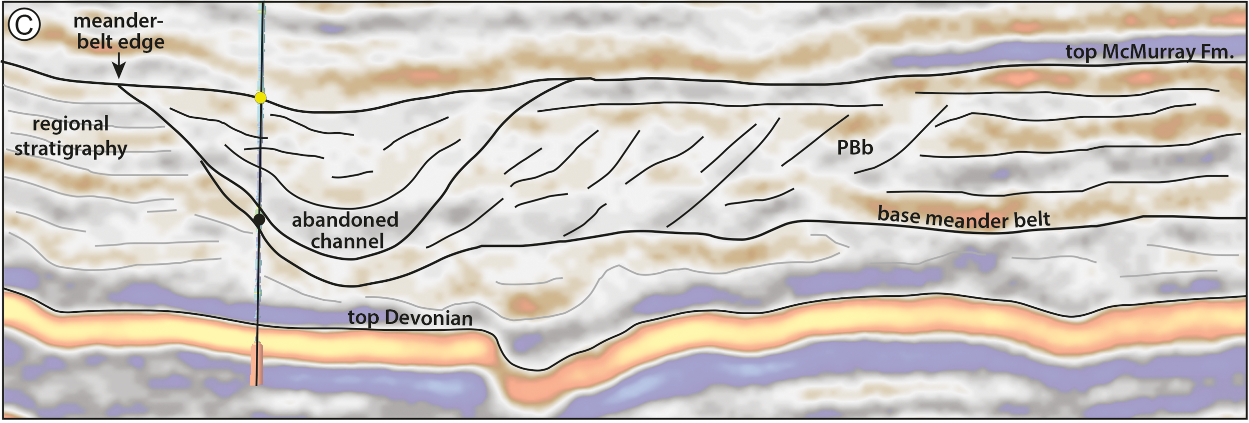
Detail from Figure 12 from Durkin et al (2017), showing a seismic section through the McMurray Formation. Most of the abandoned channels are filled with mudstone (really a siltstone). The dipping heterolithic strata of the point bars, so obvious in horizon slices, are quite subtle in section. © 2017, SEPM (Society for Sedimentary Geology) and licensed CC-BY.
The field is a geoscience wonderland. Apart from the 600 km² of beautiful 3D seismic, there are now about 1500 wells, most of which are on the 3D. In places there are more than 20 wells per section (1 sq mile, 2.6 km², 640 acres). Most of the wells have a full suite of logs, including FMI in 2/3 wells and shear sonic as well in many cases, and about 550 wells now have core through the entire reservoir interval — about 65–75 m across most of Surmont. Let that sink in for a minute.
What's so awesome about the seismic?
OK, I'm a bit biased, because I planned the acquisition of several pieces of this survey. There are some challenges to collecting great data at Surmont. The reservoir is only about 500 m below the surface. Much of the pay sand can barely be called 'rock' because it's unconsolidated sand, and the reservoir 'fluid' is a quasi-solid with a viscosity of 1 million cP. The surface has some decent topography, and the near surface is glacial till, with plenty of boulders and gravel-filled channels. There are surface lakes and the area is covered in dense forest. In short, it's a geophysical challenge.
Nonetheless, we did collect great data; here's how:
- General information
- The ca. 600 km² Supermerge consists of a dozen 3Ds recorded over about a decade starting in 2001.
- The northern 60% or so of the dataset was recombined from field records into a single 3D volume, with pre- and post-stack time imaging.
- The merge was performed by CGG Veritas, cost nearly $2 million, and took about 18 months.
- Geometry
- Most of the surveys had a 20 m shot and receiver spacing, giving the volume a 10 m by 10 m natural bin size
- The original survey had parallel and coincident shot and receiver lines (Megabin); later surveys were orthogonal.
- We varied the line spacing between 80 m and 160 m to get trace density we needed in different areas.
- Sources
- Some surveys used 125 g dynamite at a depth of 6 m; others the IVI EnviroVibe sweeping 8–230 Hz.
- We used an airgun on some of the lakes, but the data was terrible so we stopped doing it.
- Receivers
- Most of the surveys were recorded into single-point 3C digital MEMS receivers planted on the surface.
- Bandwidth
- Most of the datasets have data from about 8–10 Hz to about 180–200 Hz (and have a 1 ms sample interval).
The planning of these surveys was quite a process. Because access in the muskeg is limited to 'freeze up' (late December until March), and often curtailed by wildlife concerns (moose and elk rutting), only about 6 weeks of shooting are possible each year. This means you have to plan ahead, then mobilize a fairly large crew with as many channels as possible. After acquisition, each volume spent about 6 months in processing — mostly at Veritas and then CGG Veritas, who did fantastic work on these datasets.
Kudos to ConocoPhillips and Total for letting people work on this dataset. And kudos to Paul Durkin for this fine piece of work, and for making it open access. I'm excited to see it in the open. I hope we see more papers based on Surmont, because it may be the world's finest subsurface dataset. I hope it is released some day, it would have huge impact.
References & bibliography
Paul R. Durkin, Ron L. Boyd, Stephen M. Hubbard, Albert W. Shultz, Michael D. Blum (2017). Three-Dimensional Reconstruction of Meander-Belt Evolution, Cretaceous Mcmurray Formation, Alberta Foreland Basin, Canada. Journal of Sedimentary Research 87 (10), p 1075–1099. doi: 10.2110/jsr.2017.59 (not live yet).
Hall, M (2007). Cost-effective, fit-for-purpose, lease-wide 3D seismic at Surmont. SEG Development and Production Forum, Edmonton, Canada, July 2007.
Hall, M (2009). Lithofacies prediction from seismic, one step at a time: An example from the McMurray Formation bitumen reservoir at Surmont. Canadian Society of Exploration Geophysicists National Convention, Calgary, Canada, May 2009. Oral paper.
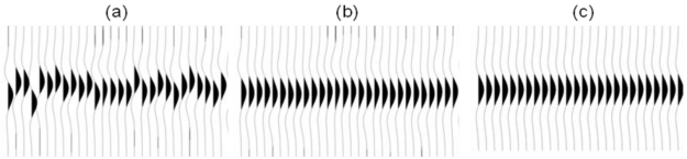
Zhu, X, S Shaw, B Roy, M Hall, M Gurch, D Whitmore and P Anno (2008). Near-surface complexity masquerades as anisotropy. SEG Annual Convention, Las Vegas, USA, November 2008. Oral paper. doi: 10.1190/1.3063976.
Surmont SAGD Performance Review (2016), by ConocoPhillips and Total geoscientists and engineers. Submitted to AER, 258 pp. Available online [PDF] — and well worth looking at.
Trad, D, M Hall, and M Cotra (2008). Reshooting a survey by 5D interpolation. Canadian Society of Exploration Geophysicists National Convention, Calgary, Canada, May 2006. Oral paper.


 Except where noted, this content is licensed