C is for clipping

Previously in our A to Z series we covered seismic amplitude and bit depth. Bit depth determines how smooth the amplitude histogram is. Clipping describes what happens when this histogram is truncated. It is often done deliberately to allow more precision for the majority of samples (in the middle of the histogram), but at the cost of no precision at all for extreme values (at the ends of the histogram). One reason to do this, for example, might be when loading 16- or 32-bit data into a software application that can only use 8-bit data (e.g. most volume interpretation software). 

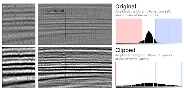
Let's look at an example. Suppose we start with a smooth, unclipped dataset represented by 2-byte integers, as in the top upper image in the figure below. Its histogram, to the right, is a close approximation to a bell curve, with no samples, or very few, at the extreme values. In a 16-bit volume, remember, these extreme values are -32 767 and +32 768. In other words, the data fit entirely within the range allowed by the bit-depth.

 Data from F3 dataset, offshore Netherlands, from the OpendTect Open Seismic Repository.

Now imagine we have to represent this data with 1-byte samples, or a bit-depth of 8. In the lower part of the figure, you see the data after this transformation with its histogram is to the right. Look at the extreme ends of the histogram: there is a big spike of samples there. All of the samples in the tails of the unclipped histogram (shown in red and blue) have been crammed into those two values: -127 and +128. For example, any sample with an amplitude of +10 000 or more in the unclipped data, now has a value of +128. Likewise, amplitudes of –10 000 or less are all now represented by a single amplitude: –127. Any nuance or subtlety in the data in those higher-magnitude samples has gone forever.

Notice the upside though: the contrast of the unclipped data has been boosted, and we might feel like we can see more detail and discriminate more features in this display. Paradoxically, there is less precision, but perhaps it's easier to interpret.

How much data did we affect? We remember to pull out our basic cheatsheet and look at the normal distribution, below. If we clip the data at about two standard deviations from the mean, then we are only affecting 4.2% of the samples in the data. This might include lots of samples of little quantitative interest (the sea-floor, for example), but is also likely to include samples you do care about: bright amplitudes in or near the zone of interest. For this reason, while clipping might not affect how you interpret the structural framework of your earth model, you need to be aware of it in any quantitative work.

Have you ever been tripped up by clipped seismic data? Do you think it should be avoided at all costs, or maybe you have a tip for avoiding severe clipping? Leave a comment!

Shale vs tight

A couple of weeks ago, we looked at definitions of unconventional resources. Two of the most important play types are shale gas and tight gas. They are volumetrically important, technologically important, and therefore economically important. Just last week, for example, Chevron bought an unconventional gas company for over $4B.

The best-known examples of shale gas plays might be the Barnett in Texas, the Marcellus in eastern US, and the Duvernay in Alberta. Tight gas plays arguably had their hyper-popular exploration boom five or so years ago, but are still experiencing huge investment in areas where they are well-understood (and have nice reservoir properties!). Prolific examples include the Bakken of northern US and the Montney of Alberta.

So if we were to generalize, perhaps over-generalize: what's the difference between shale gas plays and tight gas plays?

	Shale gas	Tight gas
Grain-size	Mostly mud	Substantially silt or fine sand
Porosity	up to 6%	up to 8%
TOC	up to 10%	up to 7%
Permeability	up to 0.001 mD	up to 1 mD
Source	Mostly self-sourced	Mostly extra-formation
Trap	None	Facies and hydrodynamic
Gas	Substantially adsorbed	Almost all in pore space
Silica	Biogenic, crypto-crystalline	Detrital quartz
Brittleness	From silica	From carbonate cement

 

Over-generalization is a problem. Have I gone too far? I have tried to indicate where the average is, but there is a space in the middle which is distinctly grey: a muddy siltstone with high TOC might have many of the characteristics in both columns; the most distal facies in the Montney are like this.

Why does this matter? Broadly speaking, the plays are developed in the same way: horizontal wells and fracture stimulation. The difference is really in how you explore for them.

Accretionary Wedge #31

This is my first contribution to the Accretionary Wedge; the theme this time is 'What geological concept or idea did you hear about that you had no notion of before (and likely surprised you in some way)?' Like most of the entries I've read so far, I could think of quite a few things fitting this description. I find lots of geological concepts surprising or counterintuitive. But in the end, I chose to write about the thing that obsessed me as an undergraduate, right at the beginning of my career:

The Devonian day was 22 hours long

In November I moved to the Atlantic coast of Canada. It's the first time I've lived right at the seaside, but I am originally from the tiny island of Great Britain so never lived too far from the edge. There is a deeply maritime feel to this part of the continent, even in the sheltered Bay of Fundy. The famously macrotidal regime there permeates the culture: artists paint the tidal landscapes; musicians sing about the eerie currents; geologists crawl around on the mud-flats and cliffs. The profound consequences of a 17-metre tidal range and its heartbeat, regular as clockwork.

← Tidal forces shape a bar-built estuary, Pamlico Sound, USA.

It's easy to see the effects of the tide in the geological record. Tidal successions are recognizable from some combination of pin-stripe lamination, mud-drapes, bi-directional ripples, proximity to shore, diagnostic fossils, brackish trace fossil assemblages, and other marvellous sedimentological tools. Less intuitively perhaps, at least for a non-biologist like me, marine animals also express these tidal frequencies in their growth patterns. So a coral, for example, might have a lunar breeding cycle. This periodicity results in growth rings just like a tree, only they record not the seasons but the bi-monthly beat of spring and neap tides. The tides are driven by the relative positions of the sun and moon relative to earth. Celestial bodies created banded coral.

From Scutton (1963): diurnal rings and and monthly bandsColin Scrutton, one of my professors at the University of Durham in the northeast of England, measured the growth ridges of rugose corals of Middle Devonian successions in Michigan, Ontario and Belgium (Scrutton 1964). He was testing the result of a similar experiment by John Wells (1963). The conclusion: the Devonian year contained 13 lunar months, each lunar month contained 30.6 days, so the year was 399 days long. According to what we know about planetary dynamics in the solar system, the year was approximately the same length so Devonian days were shorter by a couple of hours. The reason: the tides themselves, as they move westward around the eastward-spinning earth, are a simple frictional brake. The earth's rotation slows over time as the earth-moon system loses energy to heat, the ultimate entropy. Even more fascinatingly, the torque exerted by the sun is counteractive, introducing further cyclicities as these signals interfere. Day length, therefore, has probably not slowed monotonically though time.

For me, this realization was bound up with an obsession with cyclicity. I could not read enough about Milankovitch cycles: wobbles and ellipticity in the earth's dance through space scratching their pulse into the groove of the stratigraphic record and even influencing sea-floor spreading rates, perhaps even mass extinctions. The implications are profound: terametre-scale mechanics of the universe control the timing of cellular neurochemical functions.

Why anyone needs astrology to connect with this awesome fact is beyond me. 

References

Panella, G, et al (1968). Palaeontological evidence for variation in length of synodic month since late Cambrian. Science 15 (3855), p 792–796, doi: 10.1126/science.162.3855.792.
Scrutton, C (1964). Periodicity in Devonian coral growth. Palaeontology 7 (4), p 552–558, pl 86–87.
Wells, J (1963). Coral growth and geochronometry. Nature 197, p 948–950. doi: 10.1038/197948a0.

Geophysical prospecting's roots

As a schoolboy, I used to frequent the second-hand bookshops of Reading, Cambridge, and all over the south east of England. Though not much of a collector, I was taken with the challenge once: Penguin's quarterly science magazine of the late 40s and early 50s: Science News. I completed the set only a few years ago. I'll be honest, while the articles were often very interesting, I was mainly interested in the beautiful cover design. Classic mid-20th Century Penguin.

Most of the articles are very dated of course, but I find them interesting to read nonetheless. Today, I thought I'd excerpt a 1948 article by one A Harford: Advances in geophysical prospecting. It's interesting because this post-war period was really the dawn of the golden age of the oil and gas industry. Naturally, this meant rapid advances in exploration geoscience, especially well logging, reflection seismology, and gravity-magnetics. No doubt wartime technology had its effects; certainly the development of seismic and signal processing technology was accelerated by the Great War and World War II. This article is mostly about magnetic surveys, but he touches on all of these technologies.

...geophysics hardly began until the 1920’s, since when it has expanded at a furious pace. Big business found that geophysics would detect new oil-fields with greater certainty than any other means and, as they found this new technique increased their profits, they lavished money upon it for many years. As more money was spent on better instruments and interpreters the successes increased until, in fifteen years, the gravity meter for instance reached ultimate sensitivity. Between them the physicists and geologists discovered numerous oilfields with relative ease and seemed to find the pace invigorating. Certainly the oil industry has created geophysics, which even now is little used outside problems connected with oil.
DOWNLOAD THE REST OF THE ARTICLE

The blustery language ('the oil industry created geophysics'!) and fearless modernism seems quaint now, but the rate of new oil and gas discoveries at the time was several times what it is today (see chart). I sometimes wonder if the thought of technology leading us has left us jaded; one often hears people react negatively to new tools or software: "We didn't need that in my day".

← Image from Wikipedia article on peak oil

To be sure, even as a committed technologist, I love the idea of spending more money on better interpreters! Like these gentlemen geophysicists, casually examining a seismic record at Lake Arthur, Louisiana, from Harford's article:

Part of me thinks the world has changed so much—hydrocarbons are much, much harder to find today—that this is all really just ancient history. But I also recognize that the tools we have are far more powerful, and our knowledge so much more profound: plate tectonics was still a hotly-debated concept in 1948, for example. So who really has the advantage?

Disclaimer To the best of my knowledge, the original article first appeared in the October 1948 issue of Science News, published by Penguin Books of Harmondsworth, England. It is excerpted here, and made available for download, with their advice but not their explicit permission; Penguin is not involved in this website. To the best of my knowledge, the material is copyright free today; if you believe otherwise, get in touch.

How to make a strat column

A few weeks ago I posted about the brilliant TSCreator, a Java application for creating custom geological timescales. One of the nicest features of this tool is that you can create your own lithostratigraphic columns, stick charts, transgression-regression plots, isotope curves, etc. It's a slightly fiddly process, so I wanted to try to give some pointers; this post is about how to make a simple lithostrat column. The other column types are built in a similar way; the full details are described in the Manual (starting on page 20). 

The example I'm showing is the Western Cape Breton column, as given by the Nova Scotia Geological Highway Map. I can't vouch for its accuracy as I've never worked this section; I built it purely to show the method. You can see the result here >

You build the data file, which TSCreator calls a Datapack, in a spreadsheet. I use Google Docs, but you can use any tool you like (OpenOffice.org, Microsoft Excel etc), as long as it will save a tab-delimited text file. The spreadsheet has a header and a data section; here's what the header looks like in my example:

format version: 1.4
date: 10/02/2011
Chart Title: Western Cape Breton
age units: Ma

You can see my example file here (opens in Google Docs). To use it, first save it as a text file: Google Docs > File > Download as > Text. Give it a .txt extension when you get the chance. Then launch TSCreator and select File > Add Datapack. If you get an error it's probably because you have violated one of the formatting rules. It may take some back and forth to get it how you want it.

Finally, I just made the unhappy discovery that you cannot save your chart after you load a custom datapack. Apparently to export an image or SVG file (my preference), you need TS-Creator Pro. Or you get very clever with screen grabs!

If you have your own tips, please leave them in the comments!

Note, TimeScale Creator is a trademark of the Geologic TimeScale Foundation. I am not connected with the software or its creators in any way. Microsoft Excel is a trademark of Microsoft Corporation. Java is a trademark of Oracle Corporation.

Potash mine photo tour

On Friday, Matt and I went on a tour of the PCS potash mine in Penobsquis, New Brunswick, as a precursor to the 2011 Atlantic Geoscience Society Colloquium in Fredericton.

The evaporites of the Early Carboniferous Windsor Group were formed as a result of two marine incursions into an otherwise clastic red bed sequence within the Moncton sub-basin. The evaporites containing the potash ore have been folded into a NE-SW trending anticline as shown in the diagram below.

Brian Roulston hosted 24 visitors into the mine. We were lowered about 400 m down to the main workings then driven approximately 10 km underground to three main attractions: a cavern stope in the Basal Halite; an active stope in the halite; finally an active stope in the potash ore (sylvinite).

Thanks to Brian and his team at PCS for putting this tour together for us, it was so much fun.

Signage

People

Gear

Salts, rusts, colors, and textures 

Darkness

Mining the ore

Measuring value

Often in upstream oil and gas we are challenged with a simple question: what's the value? What's the value of that 3D seismic? What's the NPV of this study? How does your professional network affect our bottom line?

Sometimes, at least for me, the first reaction is indignation. Let's take the seismic example; it goes like this:

Finance guy - So, this $28M... 3D seismic. What's the value of this data set?
Geoscientist - What's the value? Of that 3D? That state-of-the-art, high-fold, wide-azimuth, long-offset, high-bandwidth, eco-friendly, ultra-safe 3D seismic survey I just spent four months designing and soliciting bids on?
Finance guy - Yeah
Geoscientist - We have four wells on twenty square kilometres of land. We want to drill forty more. The wells cost $10M each. The seismic will allow us to pick the best locations. It's 3D seismic, the best quality. We always do it. Everyone does it. We can't do subsurface science without it, not very well anyway.
Finance guy - Yeah... Sorry, what's the value of the seismic? Dollars will do.

Finance guy just wants a number. The value is clear to everyone involved. But maybe money is tight this year and finance would like to defer some costs to next year. Maybe we can lower the cost by making the survey smaller, or reducing the fold. Before too long someone utters the unspeakable: 'Value of Information'. The next month of your life becomes a frustrating spreadsheet nightmare of trying to get the process to yield the answer your team wants so you can get on with finding oil and gas.

I think there is a better way. What do you think?

The Agile* interpreter's canon

There are only two types of interpretation: those that have been revised and those that need to be.
Don Herron

As Matt mentioned before, we have been forming a concept we call agile interpretation.

Perhaps the essence of the adage "seismic interpretation is an art" suggests that there shouldn't really be a hard and fast set of rules; but having no rules begets chaos and stagnation. We think seismic interpretation is a craft. As with any craft, harnessing skill and creativity enable richer and more meaningful results. Working within a framework of principles allows one's art to flourish; paint not only with brighter, more appealing colors, but with more tailored technique for putting brush to canvas.

We have created this one-page guide as reference for seismic interpreters. Pull it out before starting, a few times in the middle, and then as a checklist or summary nearing completion of your project. We hope it's valuable for the newbie, for sorting out a plan of attack, and for seasoned veterans, to refresh work-worn concepts and tools.

We're looking to get consensus here on the things people actually do when they interpret seismic; this is very much a straw man. Maybe you have adopted some tricks that aren't obivous to the rest of us. Please leave a message in the comments section of this entry if you have any tips that would improve this handout.

Happy interpreting!