Q is for Q

Quality factor, or \(Q\), is one of the more mysterious quantities of seismology. It's right up there with Lamé's \(\lambda\) and Thomsen's \(\gamma\). For one thing, it's wrapped up with the idea of attenuation, and sometimes the terms \(Q\) and 'attenuation' are bandied about seemingly interchangeably. For another thing, people talk about it like it's really important, but it often seems to be completely ignored.

A quick aside. There's another quality factor: the rock quality factor, popular among geomechnicists (geomechanics?). That \(Q\) describes the degree and roughness of jointing in rocks, and is probably related — coincidentally if not theoretically — to seismic \(Q\) in various nonlinear and probably profound ways. I'm not going to say any more about it, but if this interests you, read Nick Barton's book, Rock Quality, Seismic Velocity, Attenuation and Anistropy (2006; CRC Press) if you can afford it. 

So what is Q exactly?

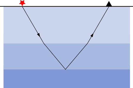
We know intuitively that seismic waves lose energy as they travel through the earth. There are three loss mechanisms: scattering (elastic losses resulting from reflections and diffractions), geometrical spreading, and intrinsic attenuation. This last one, anelastic energy loss due to absorption — essentially the deviation from perfect elasticity — is what I'm trying to describe here.

I'm not going to get very far, by the way. For the full story, start at the seminal review paper entitled \(Q\) by Leon Knopoff (1964), which surely has the shortest title of any paper in geophysics. (Knopoff also liked short abstracts, as you see here.)

The dimensionless seismic quality factor \(Q\) is defined in terms of the energy \(E\) stored in one cycle, and the change in energy — the energy dissipated in various ways, such as fluid movement (AKA 'sloshing', according to Carl Reine's essay in 52 Things... Geophysics) and intergranular frictional heat ('jostling') — over that cycle:

$$ Q \stackrel{\mathrm{def}}{=} 2 \pi \frac{E}{\Delta E} $$

Remarkably, this same definition holds for any resonator, including pendulums and electronics. Physics is awesome!

Because the right-hand side of that relationship is sort of upside down — the loss is in the denominator — it's often easier to talk about \(Q^{-1}\) which is, more or less, the percentage loss of energy in a single wavelength. This inverse of \(Q\) is proportional to the attenuation coefficient. For more details on that relationship, check out Carl Reine's essay.

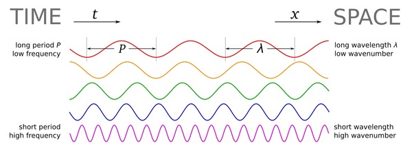
This connection with wavelengths means that we have to think about frequency. Because high frequencies have shorter cycles (by definition), they attenuate faster than low frequencies. You know this intuitively from hearing the beat, but not the melody, of distant music for example. This effect does not imply that \(Q\) depends on frequency... that's a whole other can of worms. (Confused yet?)

The frequency dependence of \(Q\)

It's thought that \(Q\) is roughly constant with respect to frequency below about 1 Hz, then increases with \(f^\alpha\), where \(\alpha\) is about 0.7, up to at least 25 Hz (I'm reading this in Mirko van der Baan's 2002 paper), and probably beyond. Most people, however, seem to throw their hands up and assume a constant \(Q\) even in the seismic bandwidth... mainly to make life easier when it comes to seismic processing. Attempting to measure, let alone compensate for, \(Q\) in seismic data is, I think it's fair to say, an unsolved problem in exploration geophysics.

Why is it worth solving? I think the main point is that, if we could model and measure it better, it could be a semi-independent measure of some rock properties we care about, especially velocity. Actually, I think it's even a stretch to call velocity a rock property — most people know that velocity depends on frequency, at least across the gulf of frequencies between seismic and acoustic logging tools, but did you know that velocity also depends on amplitude? Paul Johnson tells about this effect in his essay in the forthcoming 52 Things... Rock Physics book — stay tuned for more on that.

For a really wacky story about negative values of \(Q\) — which imply transmission coefficients greater than 1 (think about that) — check out Chris Liner's essay in the same book (or his 2014 paper in The Leading Edge). It's not going to help \(Q\) get any less mysterious, but it's a good story. Here's the punchline from a Jupyter Notebook I made a while back; it follows along with Chris's lovely paper:

Top: Velocity and the Backus average velocity in the E-38 well offshore Nova Scotia. Bottom: Layering-induced attenuation, or 1/Q, in the same well. Note the negative numbers! Reproduction of Liner's 2014 results in a Jupyter Notebook.

Top: Velocity and the Backus average velocity in the E-38 well offshore Nova Scotia. Bottom: Layering-induced attenuation, or 1/Q, in the same well. Note the negative numbers! Reproduction of Liner's 2014 results in a Jupyter Notebook.

Hm, I had hoped to shed some light on \(Q\) in this post, but I seem to have come full circle. Maybe explaining \(Q\) is another unsolved problem.

References

Barton, N (2006). Rock Quality, Seismic Velocity, Attenuation and Anisotropy. Florida, USA: CRC Press. 756 pages. ISBN 9780415394413.

Johnson, P (in press). The astonishing case of non-linear elasticity.  In: Hall, M & E Bianco (eds), 52 Things You Should Know About Rock Physics. Nova Scotia: Agile Libre, 2016, 132 pp.

Knopoff, L (1964). Q. Reviews of Geophysics 2 (4), 625–660. DOI: 10.1029/RG002i004p00625.

Reine, C (2012). Don't ignore seismic attenuation. In: Hall, M & E Bianco (eds), 52 Things You Should Know About Geophysics. Nova Scotia: Agile Libre, 2012, 132 pp.

Liner, C (2014). Long-wave elastic attenuation produced by horizontal layering. The Leading Edge 33 (6), 634–638. DOI: 10.1190/tle33060634.1. Chris also blogged about this article.

Liner, C (in press). Negative Q. In: Hall, M & E Bianco (eds), 52 Things You Should Know About Rock Physics. Nova Scotia: Agile Libre, 2016, 132 pp.

van der Bann, M (2002). Constant Q and a fractal, stratified Earth. Pure and Applied Geophysics 159 (7–8), 1707–1718. DOI: 10.1007/s00024-002-8704-0.

R is for Resolution

Resolution is becoming a catch-all term for various aspects of the quality of a digital signal, whether it's a photograph, a sound recording, or a seismic volume.

I got thinking about this on seeing an ad in AAPG Explorer magazine, announcing an 'ultra-high-resolution' 3D in the Gulf of Mexico (right), aimed at site-survey and geohazard detection. There's a nice image of the 3D, but the only evidence offered for the 'ultra-high-res' claim is the sample interval in space and time (3 m × 6 m bins and 0.25 ms sampling). This is analogous to the obsession with megapixels in digital photography, but it is only one of several ways to look at resolution. The effect of increasing the sample interval of some digital images is shown in the second column here, compared to 200 × 200 pixels originals (click to zoom):

Another aspect of resolution is spatial bandwidth, which gets at resolving power, perhaps analogous to focus for a photographer. If the range of frequencies is too narrow, then broadband features like edges cannot be represented. We can simulate poor frequency content by bandpassing the data, for example smoothing it with a Gaussian filter (column 3).

Yet another way to think about resolution is precision (column 4). Indeed, when audiophiles talk about resolution, they are talking about bit depth. We usually record seismic with 32 bits per sample, which allows us to discriminate between a large number of values — but we often view seismic with only 6 or 8 bits of precision. In the examples here, we're looking at 2 bits. Fewer bits means we can't tell the difference between some values, especially as it usually results in clipping.

If it comes down to our ability to tell events (or objects, or values) apart, then another factor enters the fray: signal-to-noise ratio. Too much noise (column 5) impairs our ability to resolve detail and discriminate between things, and to measure the true value of, say, amplitude. So while we don't normally talk about the noise level as a resolution issue, it is one. And it may have the most variety: in seismic acquisition we suffer from thermal noise, line noise, wind and helicopters, coherent noise, and so on.

I can only think of one more impairment to the signals we collect, and it may be the most troubling: the total duration or extent of the observation (column 6). How much information can you afford to gather? Uncertainty resulting from a small window is the basis of the game Name That Tune. If the scale of observation is not appropriate to the scale we're interested in, we risk a kind of interpretation 'gap' — related to a concept we've touched on before — and it's why geologists' brains need to be helicoptery. A small 3D is harder to interpret than a large one. 

The final consideration is not a signal effect at all. It has to do with the nature of the target itself. Notice how tolerant the brick wall image is to the various impairments (especially if you know what it is), and how intolerant the photomicrograph is. In the astronomical image, the galaxy is tolerant; the stars are not. Notice too that trying to 'resolve' the galaxy (into a point, say) would be a mistake: it is inherently low-resolution. Indeed, its fuzziness is one of its salient features.

Have I missed anything? Are there other ways in which the recorded signal can suffer and targets can be confused or otherwise unresolved? How does illumination fit in here, or spectral bandwidth? What do you mean when you talk about resolution?


This post is an exceprt from my talk at SEG, which you can read about in this blog post. You can even listen to it if you're really bored. The images were generated by one of my IPython Notebooks that I point to in the talk, specifically images.ipynb

Astute readers with potent memories will have noticed that we have skipped Q in our A to Z. I just cannot seem to finish my post about Q, but I will!

The Safe Band ad is copyright of NCS SubSea. This low-res snippet qualifies as fair use for comment.

P is for Phase

Seismic is about acoustic vibration. The archetypal oscillation, the sine wave, describes the displacement y of a point around a circle. You only need three pieces of information to describe it perfectly: the size of the circle, the speed at which it rotates around the circle, and where it starts from expressed as an angle. These quantities are better known as the amplitude, frequency, and phase respectively. These figures show how varying each of them affects the waveform:

So phase describes the starting point as an angle, but notice that this manifests itself as an apparent lateral shift in the waveform. For seismic data, this means a time shift. More on this later. 

What about seismic?

We know seismic signals are not so simple — they are not repetitive oscillations — so why do the words amplitudefrequency and phase show up so often? Aren't these words horribly inadequate?

Not exactly. Fourier's methods allow us to construct (and deconstruct) more complicated signals by adding up a series of sine waves, as long as we get the amplitude, frequency and phase values right for each one of them. The tricky part, and where much of where the confusion lies, is that even though you can place your finger on any point along a seismic trace and read off a value for amplitude, you can't do that for frequency or phase. The information for those are only unlocked through spectroscopy.

Phase shifts or time shifts?

The Ricker wavelet is popular because it can easily be written analytically, and it is comprised of a considerable number of sinusoids of varying amplitudes and frequencies. We might refer to a '20 Hz Ricker wavelet' but really it contains a range of frequencies. The blue curve shows the wavelet with phase = 0°, the purple curve shows the wavelet with a phase shift of π/3 = 60° (across all frequencies). Notice how the frequency content remains unchanged.

So for a seismic reflection event (below), phase takes on a new meaning. It expresses a time offset between the reflection and the maximum value on the waveform. When the amplitude maximum is centered at the reflecting point, it is equally shaped on either side — we call this zero phase. Notice how variations in the phase of the event alter the relative position of the peak and sidelobes. The maximum amplitude of the event at 90° is only about 80% of the amplitude at zero phase. This is why I like to plot traces along with their envelope (the grey lines). The envelope contains all possible phase rotations. Any event whose maximum value does not align with the maximum on the envelope is not zero phase.

Understanding the role of phase in time series analysis is crucial for both data processors aiming to create reliable data, and interpreters who operate under the assertion that subtle variations in waveform shape can be attributed to underlying geology. Waveform classification is a powerful attribute... but how reliable is it?

In a future post, I will cover the concept of instantaneous phase on maps and sections, and some other practical interpretation tips. If you have any of your own, share them in the comments.

Additional reading
Liner, C (2002). Phase, phase, phase. The Leading Edge 21, p 456–7. Abstract online.

O is for Offset

Offset is one of those jargon words that geophysicists kick around without a second thought, but which might bewilder more geological interpreters. Like most jargon words, offset can mean a couple of different things: 

  • Offset distance, which is usually what is meant by simply 'offset'.
  • Offset angle, which is often what we really care about.
  • We are not talking about offset wells, or fault offset.

What is offset?

Sherriff's Encyclopedic Dictionary is characteristically terse:

Offset: The distance from the source point to a geophone or to the center of a geophone group.

The concept of offset only really makes sense in the pre-stack world — to field data and gathers. The traces in stacked data (everyday seismic volumes) combine data from many offsets. So let's look at the geometry of seismic acquisition. A map shows the layout of shots (red) and receivers (blue). We can define offset and azimuth A at the midpoint of every shot–receiver pair, on a map (centre) and in section (right):

Offset distance applies to traces. The offset distance is the straight-line distance from the vibrator, shot-hole or air-gun (or any other source) to the particular receiver that recorded the trace in question. If we know the geometry of the acquisition, and the size of the recording patch or length of the streamers, then we can calculate offset distance exactly. 

Offset angle applies to specific samples on a trace. The offset angle is the incident angle of the reflected ray that that a given sample represents. Samples at the top of a trace have larger offset angles than those at the bottom, even though they have the same offset distance. To compute these angles, we need to know the vertical distances, and this requires knowledge of the velocity field, which is mostly unknown. So offset angle is not objective, but a partly interpreted quantity.

Why do we care?

Acquiring longer offsets can help undershoot gaps in a survey, or image beneath salt canopies and other recumbent features. Longer offsets also helps with velocity estimation, because we see more moveout.

Looking at how the amplitude of a reflection changes with offset is the basis of AVO analysis. AVO analysis, in turn, is the basis of many fluid and lithology prediction techniques.

Offset is one of the five canonical dimensions of pre-stack seismic data, along with inline, crossline, azimuth, and frequency. As such, it is a key part of the search for sparsity in the 5D interpolation method perfected by Daniel Trad at CGGVeritas. 

Recently, geophysicists have become interested not just in the angle of a reflection, but in the orientation of a reflection too. This is because, in some geological circumstances, the amplitude of a reflection depends on the orientation with respect to the compass, as well as the incidence angle. For example, looking at data in both of these dimensions can help us understand the earth's stress field.

Offset is the characteristic attribute of pre-stack seismic data. Seismic data would be nothing without it.

N is for Nyquist

In yesterday's post, I covered a few ideas from Fourier analysis for synthesizing and processing information. It serves as a primer for the next letter in our A to Z blog series: N is for Nyquist.

In seismology, the goal is to propagate a broadband impulse into the subsurface, and measure the reflected wavetrain that returns from the series of rock boundaries. A question that concerns the seismic experiment is: What sample rate should I choose to adequately capture the information from all the sinusoids that comprise the waveform? Sampling is the capturing of discrete data points from the continuous analog signal — a necessary step in recording digital data. Oversample it, using too high a sample rate, and you might run out of disk space. Undersample it and your recording will suffer from aliasing.

What is aliasing?

Aliasing is a phenomenon observed when the sample interval is not sufficiently brief to capture the higher range of frequencies in a signal. In order to avoid aliasing, each constituent frequency has to be sampled at least two times per wavelength. So the term Nyquist frequency is defined as half of the sampling frequency of a digital recording system. Nyquist has to be higher than all of the frequencies in the observed signal to allow perfect recontstruction of the signal from the samples.

Above Nyquist, the signal frequencies are not sampled twice per wavelength, and will experience a folding about Nyquist to low frequencies. So not obeying Nyquist gives a double blow, not only does it fail to record all the frequencies, the frequencies that you leave out actually destroy part of the frequencies you do record. Can you see this happening in the seismic reflection trace shown below? You may need to traverse back and forth between the time domain and frequency domain representation of this signal.

Nyquist_trace.png

Seismic data is usually acquired with either a 4 millisecond sample interval (250 Hz sample rate) if you are offshore, or 2 millisecond sample interval (500 Hz) if you are on land. A recording system with a 250 Hz sample rate has a Nyquist frequency of 125 Hz. So information coming in above 150 Hz will wrap around or fold to 100 Hz, and so on. 

It's important to note that the sampling rate of the recording system has nothing to do the native frequencies being observed. It turns out that most seismic acquisition systems are safe with Nyquist at 125 Hz, because seismic sources such as Vibroseis and dynamite don't send high frequencies very far; the earth filters and attenuates them out before they arrive at the receiver.

Space alias

Aliasing can happen in space, as well as in time. When the pixels in this image are larger than half the width of the bricks, we see these beautiful curved artifacts. In this case, the aliasing patterns are created by the very subtle perspective warping of the curved bricks across a regularly sampled grid of pixels. It creates a powerful illusion, a wonderful distortion of reality. The observations were not sampled at a high enough rate to adequately capture the nature of reality. Watch for this kind of thing on seismic records and sections. Spatial alaising. 

Click for the full demonstration (or adjust your screen resolution).You may also have seen this dizzying illusion of an accelerating wheel that suddenly appears to change direction after it rotates faster than the sample rate of the video frames captured. The classic example is the wagon whel effect in old Western movies.

Aliasing is just one phenomenon to worry about when transmitting and processing geophysical signals. After-the-fact tricks like anti-aliasing filters are sometimes employed, but if you really care about recovering all the information that the earth is spitting out at you, you probably need to oversample. At least two times for the shortest wavelengths.

M is for Migration

One of my favourite phrases in geophysics is the seismic experiment. I think we call it that to remind everyone, especially ourselves, that this is science: it's an experiment, it will yield results, and we must interpret those results. We are not observing anything, or remote sensing, or otherwise peering into the earth. When seismic processors talk about imaging, they mean image construction, not image capture

The classic cartoon of the seismic experiment shows flat geology. Rays go down, rays refract and reflect, rays come back up. Simple. If you know the acoustic properties of the medium—the speed of sound—and you know the locations of the source and receiver, then you know where a given reflection came from. Easy!

But... some geologists think that the rocks beneath the earth's surface are not flat. Some geologists think there are tilted beds and faults and big folds all over the place. And, more devastating still, we just don't know what the geometries are. All of this means trouble for the geophysicist, because now the reflection could have come from an infinite number of places. This makes choosing a finite number of well locations more of a challenge. 

What to do? This is a hard problem. Our solution is arm-wavingly called imaging. We wish to reconstruct an image of the subsurface, using only our data and our sharp intellects. And computers. Lots of those.

Imaging with geometry

Agile's good friend Brian Russell wrote one of my favourite papers (Russell, 1998) — an imaging tutorial. Please read it (grab some graph paper first). He walks us through a simple problem: imaging a single dipping reflector.

Remember that in the seismic experiment, all we know is the location of the shots and receivers, and the travel time of a sound wave from one to the other. We do not know the reflection points in the earth. If we assume dipping geology, we can use the NMO equation to compute the locus of all possible reflection points, because we know the travel time from shot to receiver. Solutions to the NMO equation — given source–receiver distance, travel time, and the speed of sound — thus give the ellipse of possible reflection points, shown here in blue:

Clearly, knowing all possible reflection points is interesting, but not very useful. We want to know which reflection point our recorded echo came from. It turns out we can do something quite easy, if we have plenty of data. Fortunately, we geophysicists always bring lots and lots of receivers along to the seismic experiment. Thousands usually. So we got data.

Now for the magic. Remember Huygens' principle? It says we can imagine a wavefront as a series of little secondary waves, the sum of which shows us what happens to the wavefront. We can apply this idea to the problem of the tilted bed. We have lots of little wavefronts — one for each receiver. Instead of trying to figure out the location of each reflection point, we just compute all possible reflection points, for all receivers, then add them all up. The wavefronts add constructively at the reflector, and we get the solution to the imaging problem. It's kind of a miracle. 

Try it yourself. Brian Russell's little exercise is (geeky) fun. It will take you about an hour. If you're not a geophysicist, and even if you are, I guarantee you will learn something about how the miracle of the seismic experiment. 

Reference
Russell, B (1998). A simple seismic imaging exercise. The Leading Edge 17 (7), 885–889. DOI: 10.1190/1.1438059

L is for Lambda

Hooke's law says that the force F exerted by a spring depends only on its displacement x from equilibrium, and the spring constant k of the spring:

.

We can think of k—and experience it—as stiffness. The spring constant is a property of the spring. In a sense, it is the spring. Rocks are like springs, in that they have some elasticity. We'd like to know the spring constant of our rocks, because it can help us predict useful things like porosity. 

Hooke's law is the basis for elasticity theory, in which we express the law as

stress [force per unit area] is equal to strain [deformation] times a constant

This time the constant of proportionality is called the elastic modulus. And there isn't just one of them. Why more complicated? Well, rocks are like springs, but they are three dimensional.

In three dimensions, assuming isotropy, the shear modulus μ plays the role of the spring constant for shear waves. But for compressional waves we need λ+2μ, a quantity called the P-wave modulus. So λ is one part of the term that tells us how rocks get squished by P-waves.

These mysterious quantities λ and µ are Lamé's first and second parameters. They are intrinsic properties of all materials, including rocks. Like all elastic moduli, they have units of force per unit area, or pascals [Pa].

So what is λ?

Matt and I have spent several hours discussing how to describe lambda. Unlike Young's modulus E, or Poisson's ratio ν, our friend λ does not have a simple physical description. Young's modulus just determines how much longer something gets when I stretch it. Poisson's ratio tells how much fatter something gets if I squeeze it. But lambda... what is lambda?

  • λ is sometimes called incompressibility, a name best avoided because it's sometimes also used for the bulk modulus, K.  
  • If we apply stress σ1 along the 1 direction to this linearly elastic isotropic cube (right), then λ represents the 'spring constant' that scales the strain ε along the directions perpendicular to the applied stress.
  • The derivation of Hooke's law in 3D requires tensors, which we're not getting into here. The point is that λ and μ help give the simplest form of the equations (right, shown for one dimension).

The significance of elastic properties is that they determine how a material is temporarily deformed by a passing seismic wave. Shear waves propagate by orthogonal displacements relative to the propagation direction—this deformation is determined by µ. In contrast, P-waves propagate by displacements parallel to the propagation direction, and this deformation is inversely proportional to M, which is 2µ + λ

Lambda rears its head in seismic petrophysics, AVO inversion, and is the first letter in the acronym of Bill Goodway's popular LMR inversion method (Goodway, 2001). Even though it is fundamental to seismic, there's no doubt that λ is not intuitively understood by most geoscientists. Have you ever tried to explain lambda to someone? What description of λ do you find useful? I'm open to suggestions. 

Goodway, B., 2001, AVO and Lame' constants for rock parameterization and fluid detection: CSEG Recorder, 26, no. 6, 39-60.

K is for Wavenumber

Wavenumber, sometimes called the propagation number, is in broad terms a measure of spatial scale. It can be thought of as a spatial analog to the temporal frequency, and is often called spatial frequency. It is often defined as the number of wavelengths per unit distance, or in terms of wavelength, λ:

$$k = \frac{1}{\lambda}$$

The units are \(\mathrm{m}^{–1}\), which are nameless in the International System, though \(\mathrm{cm}^{–1}\) are called kaysers in the cgs system. The concept is analogous to frequency \(f\), measured in \(\mathrm{s}^{–1}\) or Hertz, which is the reciprocal of period \(T\); that is, \(f = 1/T\). In a sense, period can be thought of as a temporal 'wavelength' — the length of an oscillation in time.

If you've explored the applications of frequency in geophysics, you'll have noticed that we sometimes don't use ordinary frequency f, in Hertz. Because geophysics deals with oscillating waveforms, ones that vary around a central value (think of a wiggle trace of seismic data), we often use the angular frequency. This way we can also express the close relationship between frequency and phase, which is an angle. So in many geophysical applications, we want the angular wavenumber. It is expressed in radians per metre:

$$k = \frac{2\pi}{\lambda}$$

The relationship between angular wavenumber and angular frequency is analogous to that between wavelength and ordinary frequency — they are related by the velocity V:

$$k = \frac{\omega}{V}$$

It's unfortunate that there are two definitions of wavenumber. Some people reserve the term spatial frequency for the ordinary wavenumber, or use ν (that's a Greek nu, not a vee — another potential source of confusion!), or even σ for it. But just as many call it the wavenumber and use k, so the only sure way through the jargon is to specify what you mean by the terms you use. As usual!

Just as for temporal frequency, the portal to wavenumber is the Fourier transform, computed along each spatial axis. Here are two images and their 2D spectra — a photo of some ripples, a binary image of some particles, and their fast Fourier transforms. Notice how the more organized image has a more organized spectrum (as well as some artifacts from post-processing on the image), while the noisy image's spectrum is nearly 'white':

Explore our other posts about scale.

The particle image is from the sample images in FIJI. The FFTs were produced in FIJI.

Update

on 2012-05-03 16:41 by Matt Hall

Following up on Brian's suggesstion in the comments, I added a brief workflow to the SubSurfWiki page on wavenumber. Please feel free to add to it or correct it if I messed anything up. 

J is for Journal

I'm aware of a few round-ups of journals for geologists, but none for those of us with more geophysical leanings. So here's a list of some of the publications that used to be on my reading list back when I used to actually read things. I've tried to categorize them a bit, but this turned out to be trickier than I thought it would be; I hope my buckets make some sense.

Journals with mirrored content at GeoScienceWorld are indicated by GSW

Peer-reviewed journals

Technical magazines

  • First Break — indispensible news from EAGE and the global petroleum scene, and a beautifully produced periodical to boot. No RSS feed, though. Boo. Subscription only.
  • The Leading EdgeGSWRSS — SEG's classic monthly that You Must Read. But... subscription only.
  • Recorder is brilliant value for money, even if it doesn't have an RSS feed. It is also publicly accessible after three months, which is rare to see in our field. Yay, CSEG!

Other petroleum geoscience readables

  • SPE Journal of Petroleum Technology — all the news you need from SPE. It's all online if you can bear the e-reader interface. Mostly manages to tread the marketing-as-article line that some other magazines transgress more often (none of those here; you know what they are).
  • CWLS InSite — openly accessible and often has excellent articles, though it only comes out twice a year now. Its sister organisation, SPWLA, allegedly has a journal called Petrophysics, but I've never seen it and can't find it online. Anyone?
  • Elsevier publish a number of excellent journals, but as you may know, a large part of the scientific community is pressuring the Dutch publishing giant to adopt a less exclusive distribution and pricing model for its content. So I am not reading them any more, or linking to them today. This might seem churlish, but consider that it's not uncommon to be asked for $40 per article, even if the research was publicly funded.

General interest magazines

  • IEEE SpectrumRSS — a terrific monthly from 'the world's largest association for the advancement of technology'. They also publish some awesome niche titles like the unbelievably geeky Signal Processing — RSS. You can subscribe to print issues of Spectrum without joining IEEE, and it's free to read online. My favourite.
  • Royal Statistical Society SignificanceRSS (seems to be empty) — another fantastic cross-disciplinary read. [Updated: You don't have to join the society to get it, and you can read everything online for free]. I've happily paid for this for many years.

How do I read all this stuff?

The easiest way is to grab the RSS feed addresses (right-click and Copy Link Address, or words to that effect) and put them in a feed reader like Google Reader. (Confused? What the heck is RSS?). If you prefer to get things in your email inbox, you can send RSS feeds to email.

If you read other publications that help you stay informed and inspired as an exploration geophysicist — or as any kind of subsurface scientist — let us know what's in your mailbox or RSS feed!

The cover images are copyright of CSEG, CWLS and IEEE. I'm claiming 'fair use' for these low-res images. More A to Z posts...

I is for integrated trace

A zero-phase wavelet has peaks and troughs that line up with interfaces, and has side-lobe events not associated with physical boundaries. Because of this, we see that seismic amplitude is only, at best, a proxy for earth's material contrasts (as shown below by the impedance log) and can be difficult to interpret. The largest positive amplitude corresponds to a downward increase in impedance, and the largest negative amplitude corresponds to a downward decrease in impedance.

Now consider the integral of the seismic trace. In the illustration, I have coloured the positive amplitude values blue, and the negative amplitude values red, for each time sample. The integral is literally the sample-by-sample cumulative sum of amplitudes. Notice how the shape of the trace integral now looks similar to the impedance log (far left). The inflections correlate to the bed boundaries; the integration has done a 90 degree phase rotation of the data. The integrated trace looks more like the geologic contrasts. To think of it another way, if the derivative of impedance is reflectivity, then the derivative of the integrated trace is the seismic trace.  

Impedance_Int_tr_Inversion.png

In the final column on the right, the integrated trace has been scaled so that the relative variations approximately match the absolute variations of the actual acoustic impedance log. This curve is merely a squeeze and bulkshift of the integrated trace, to align with the impedance of the background lithology. In practice, scaling seismic measurements to geologically realistic ranges requires the knowledge of rock properties from nearby well logs. The trace on the far right is a rudimentary geology-from-seismic transformation of the data. Although the general shape of the 3-layer model is reconstructed, there are some complications. The first and third layer is too soft, the middle layer is too hard (and wobbly). The appearance of a high impedance doublet is because the seismic is band-limited. 

It is important to note that a trace integral does not yield a seismic estimate of impedance, it is only a proxy. Consider it a starting point for seismic inversion, not a substitute for it. In oil sands, for instance, Matt showed how the integrated trace gives a considerably more robust estimate of impedance for reservoir characterization compared to a more time consuming and expensive seismic inversion process.

Integrated trace is not meant to be the final product in a reservoir characterization workflow, but it is a seismic attribute that you should be working with anytime you are are trying to do inversion. It should be a starting point, a sanity check, because it is fast to run, easy to understand, completely deterministic (no guess work). If it is not available on your standard interpretation software, Geocraft is one place where you can do it.