What is the fastest axis of an array?

One of the participants in our geocomputing course asked us a tricky question earlier this year. She was a C++ and Java programmer — we often teach experienced programmers who want to learn about Python and/or machine learning — and she worked mostly with seismic data. She had a question related to the performance of n-dimensional arrays: what is the fastest axis of a NumPy array?

I’ve written before about how computational geoscience is not ‘software engineering’ and not ‘computer science’, but something else. And there’s a well established principle in programming, first expressed by Michael Jackson:

We follow two rules in the matter of optimization:
Rule 1: Don’t do it.
Rule 2 (for experts only). Don’t do it yet — that is, not until you have a perfectly clear and unoptimized solution.

Most of the time the computer is much faster than we need it to be, so we don’t spend too much time thinking about making our programs faster. We’re mostly concerned with making them work, then making them correct. But sometimes we have to think about speed. And sometimes that means writing smarter code. (Other times it means buying another GPU.) If your computer spends its days looping over seismic volumes extracting slices for processing, you should probably know whether you want to put time in the first dimension or the last dimension of your array.

The 2D case

Let’s think about a two-dimensional case first — imagine a small 2D array, also known as a matrix in some contexts. I’ve coloured in the elements of the matrix to make the next bit easier to understand.

matrix-memory-a.png

When we store a matrix in a computer (or an image, or any array), we have a decision to make. In simple terms, the computer’s memory is like a long row of boxes, each with a unique address — shown here as a 3-digit hexadecimal number:

We can only store one number in each box, so we’re going to have to flatten the 2D array. The question is, do we put the rows in together, effectively splitting up the columns, or do we put the columns in together? These two options are commonly known as ‘row major’, or C-style, and ‘column major’, or Fortran-style:

matrix-memory-b.png

Let’s see what this looks like in terms of the indices of the elements. We can plot the index number on each axis vs. the position of the element in memory. Notice that the C-ordered elements are contiguous in axis 0:

If you spend a lot of time loading seismic data, you probably recognize this issue — it’s analgous to how traces are stored in a SEG-Y file. Of couse, with seismic data, two dimensions aren’t always enough…

Higher dimensions

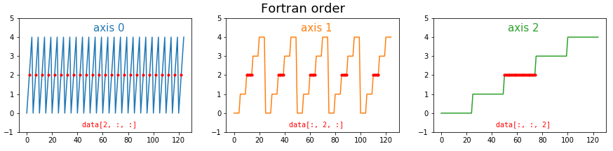
The problem multiplies at higher dimensions. If we have a cube of data, then C-style ordering results in the first dimension having large contiguous chunks, and the last dimension being broken up. The middle dimension is somewhere in between. As before, we can illustrating this by plotting the indices of the data. This time I’m highlighting the positions of the elements with index 2 (i.e. the third element) in each dimension:

So if this was a seismic volume, we might organize inlines in the first dimension, and travel-time in the last dimension. That way, we can access inlines very quickly, but timeslices will take longer.

In Fortran order, which we can optionally specify in NumPy, the situation is reversed. Now the fast axis is the last axis:

3d-array-forder.png

Lots of programming languages and libraries use row-major memory layout, including C, C++, Torch and NumPy. Most others use column-major ordering, including MATLAB, R, Julia, and Fortran. (Some other languages, such as Java and .NET, use a variant of row-major order called Iliffe vectors). NumPy calls row-major order ‘C’ (for C, not for column), and column-major ‘F’ for Fortran (thankfully they didn’t use R, for R not for row).

I expect it’s related to their heritage, but the Fortran-style languages also start counting at 1, whereas the C-style languages, including Python, start at 0.

What difference does it make?

The main practical difference is in the time it takes to access elements in different orientations. It’s faster for the computer to take a contiguous chunk of neighbours from the memory ‘boxes’ than it is to have to ‘stride’ across the memory taking elements from here and there.

How much faster? To find out, I made datasets full of random numbers, then selected slices and added 1 to them. This was the simplest operation I could think of that actually forces NumPy to do something with the data. Here are some statistics — the absolute times are pretty irrelevant as the data volumes I used are all different sizes, and the speeds will vary on different machines and architectures:

  • 2D data: 3.6× faster. Axis 0: 24.4 µs, axis 1: 88.1 µs (times relative to first axis: 1, 3.6).

  • 3D data: 43× faster. 229 µs, 714 µs, 9750 µs (relatively 1, 3.1, 43).

  • 4D data: 24× faster. 1.27 ms, 1.36 ms, 4.77 ms, 30 ms (relatively 1, 1.07, 3.75, 23.6).

  • 5D data: 20× faster. 3.02 ms, 3.07 ms, 5.42 ms, 11.1 ms, 61.3 ms (relatively 1, 1.02, 1.79, 3.67, 20.3).

  • 6D data: 5.5× faster. 24.4 ms, 23.9 ms, 24.1 ms, 37.8 ms, 55.3 ms, 136 ms (relatively 1, 0.98, 0.99, 1.55, 2.27, 5.57).

These figures are more or less simply reversed for Fortran-ordered arrays (see the notebook for datails).

Clearly, the biggest difference is with 3D data, so if you are manipulating seismic data a lot and need to access the data in that last dimension, usually travel-time, you might want to think about ways to reduce this overhead.

What difference does it really make?

The good news is that, for most of us most of the time, we don’t have to worry about any of this. For one thing, NumPy’s internal workings (in particular, its universal functions, or ufuncs) know which directions are fastest and take advantage of this when possible. For another thing, we generally try to avoid looping over arrays at all, leaving the iterative components of our algorithms to the ufuncs — so the slicing speed isn’t a factor. Even when it is a factor, or if we can’t avoid looping, it’s often not the bottleneck in the code. Usually the guts of our algorithm are what are slowing the computer down, not the access to memory. The net result of all this is that we don’t often have to think about the memory layout of our arrays.

So when does it matter? The following situations merit a bit of thought:

  • When you’re doing a very large number of accesses to memory or disk. Saving a few microseconds might add up to a lot if you’re doing it a billion times.

  • When the objects you’re accessing are very large. Reading and writing elements of a 200GB array in memory brings new challenges compared to handling a few gigabytes.

  • Reading and writing data files — really just another kind of memory — brings all the same issues. Reading a chunk of contiguous data is much faster than reading bytes from here and there. Landmark’s BRI seismic data format, Schlumberger’s ZGY files, and HDF5 files, all implement strategies to help make reading arbitrary data faster.

  • Converting code from other languages, especially MATLAB, although do realize that other languages may have their own indexing rules, as well as differing in how they store n-dimensional arrays.

If you determine that you do need to think about this stuff, then you’re going to need to read this essay about NumPy’s internal representations, and I recommend checking out this blog post by Eli Bendersky too.

There you have it. Very occasionally we scientists also need to think a bit about how computers work… but most of the time someone has done that thinking for us.

Some of the figures and all of the timings for this post came from this notebook — please have a look. If you have anything to add, or (better yet) correct, please get in touch. I’d love to hear from you.

2018 retrospective

It’s almost the end of another trip around the sun. I hope it’s been kind to you. I mean, I know it’s sometimes hard to see the kindness for all the nonsense and nefariousness in <ahem> certain parts of the world, but I hope 2018 at least didn’t poke its finger in your eye, or set fire to any of your belongings. If it did — may 2019 bring you some eye drops and a fire extinguisher.

Anyway, at this time of year, I like to take a quick look over my shoulder at the past 12 months. Since I’m the over-sharing type, I like to write down what I see and put it on the Internet. I apologize, and/or you’re welcome.

Top of the posts

We’ve been busier than ever this year, and the blog has taken a bit of a hit. In spite of the reduced activity (only 45 posts, compared to 53 last year), traffic continues to grow and currently averages 9000 unique visitors per month. These were the most visited posts in 2018:

Last December’s post, No more rainbows, got more traffic this year than any of these posts. And, yet again, k is for wavenumber got more than any. What is it with that post??

Where in the world?

Every year I take a look at where our people are reading the blog from (according to Google). We’ve travelled more than usual this year too, so I’ve added our various destinations to the map… it makes me realize we’re still missing most of you.

blog-map-2018.png
  1. Houston (number 1 last year)

  2. London (up from 3)

  3. Calgary (down from 2)

  4. Stavanger (6)

  5. Paris (9)

  6. New York (—)

  7. Perth (4)

  8. Bangalore (—)

  9. Jakarta (—)

  10. Kuala Lumpur (8)

Together these cities capture at least 15% of our readship. New York might be an anomaly related to the location of cloud infrastructure there. (Boardman, Oregon, shows up for the same reason.) But who knows what any of these numbers mean…

Work

People often ask us how we earn a living, and sometime I wonder myself. But not this year: there was a clear role for us to play in 2018 — training the next wave of digital scientists and engineers in subsurface.

Rob.jpeg
  • We continued the machine learning project on GPR interpretation that we started last year.

  • We revived Pick This and have it running on a private corporate cloud at a major oil company, as well as on the Internet.

  • We have spent 63 days in the classroom this year, and taught 325 geoscientists the fundamentals of Python and machine learning.

  • Apart from the 6 events of our own that we organized, we were involved in 3 other public hackathons and 2 in-house hackathons.

  • We hired awesome digital geologist Robert Leckenby (right) full time. 

The large number of people we’re training at the moment is especially exciting, because of what it means for the community. We spent 18 days in the classroom and trained 139 scientists in the previous four years combined — so it’s clear that digital geoscience is important to people today. I cannot wait to see what these new coders do in 2019 and beyond!

The hackathon trend is similar: we hosted 310 scientists and engineers this year, compared to 183 in the four years from 2013 to 2017. Numbers are only numbers of course, but the reality is that we’re seeing more mature projects, and more capable coders, at every event. I know it’s corny to say so, but I feel so lucky to be a scientist today, there is just so much to do.

Cheers to you

Agile is, as they say, only wee. And we all live in far-flung places. But the Intertubes are a marvellous thing, and every week we meet new people and have new conversations via this blog, and on Twitter, and the Software Underground. We love our community, and are grateful to be part of it. So thank you for seeking us out, cheering us on, hiring us, and just generally being a good sport about things.

From all of us at Agile, have a fantastic festive season — and may the new year bring you peace and happiness.

The London hackathon

At the end of November I reported on the projects at the Oil & Gas Authority’s machine learning hackathon in Aberdeen. This post is about the follow-up event at London Olympia.


Like the Aberdeen hackathon the previous weekend, the theme was ‘machine learning’. The event unfolded in the Apex Room at Olympia, during the weekend before the PETEX conference. The venue was excellent, with attentive staff and top-notch catering. Thank you to the PESGB for organizing that side of things.

Thirty-eight digital geoscientists spent the weekend with us, and most of them also took advantage of the bootcamp on Friday; at least a dozen of those had not coded at all before the event. It’s such a privilege to work with people on their skills at these events, and to see them writing their own code over the weekend.

Here’s the full list of projects from the event…


Sweet spot hunting

Sweet Spot Sweat Shop: Alan Wilson, Geoff Chambers, Marco van der Linden, Maxim Kotenev, Rowan Haddad.

Project: We’ve seen a few people tackling the issue of making decisions from large numbers of realizations recently. The approach here was to generate maps of various outputs from dynamic modeling and present these to the user in an interactive way. The team also had maps of sweet spots, as determined by simulation, and they attempted to train models to predict these sweetspots directly from the property maps. The result was a unique and interesting exploration of the potential for machine learning to augment standard workflows in reservoir modeling and simulation. Project page. GitHub repo.

sweetspot_prediction.png

An intelligent dashboard

Dash AI: Vincent Penasse, Pierre Guilpain.

Project: Vincent and Pierre believed so strongly in their project that they ran with it as a pair. They started with labelled production history from 8 wells in a Pandas dataframe. They trained some models, including decision trees and KNN classifiers, to recognizedata issues and recommend required actions. Using skills they gained in the bootcamp, they put a flask web app in front of these to allow some interaction. The result was the start of an intelligent dashboard that not only flagged issues, but also recommended a response. Project page.

This project won recognition for impact.

DashAI-team.jpg

Predicting logs ahead of the bit

Team Mystic Bit: Connor Tann, Lawrie Cowliff, Justin Boylan-Toomey, Patrick Davies, Alessandro Christofori, Dan Austin, Jeremy Fortun.

Project: Thinking of this awesome demo, I threw down the gauntlet of real-time look-ahead prediction on the Friday evening, and Connor and the Mystic Bit team picked it up. They did a great job, training a series of models to predict a most likely log (see right) as well as upper and lower bounds. In the figure, the bit is currently at 1770 m. The model is shown the points above this. The orange crosses are the P90, P50 and P10 predictions up to 40 m ahead of the bit. The blue points below 1770 m have not yet been encountered. Project page. GitHub repo.

This project won recognition for best execution.

MysticBit_log-pred.png

The seals make a comeback

Selkie Se7en: Georgina Malas, Matthew Gelsthorpe, Caroline White, Karen Guldbaek Schmidt, Jalil Nasseri, Joshua Fernandes, Max Coussens, Samuel Eckford.

Project: At the Aberdeen hackathon, Julien Moreau brought along a couple of satellite image with the locations of thousands of seals on the images. They succeeded in training a model to correctly identify seal locations 80% of the time. In London, another team of almost all geologists picked up the project. They applied various models to the task, and eventually achieved a binary prediction accuracy of over 97%. In addition, the team trained a multiclass convolutional neural network to distinguish between whitecoats (pups), moulted seals (yearlings and adults), double seals, and dead seals.

Impressive stuff; it’s always inspiring to see people operating way outside their comfort zone. Project page.

selkie-seven.png

Interpreting the language of stratigraphy

The Lithographers: Gijs Straathof, Michael Steventon, Rodolfo Oliveira, Fabio Contreras, Simon Franchini, Malgorzata Drwila.

Project: At the project bazaar on Friday (the kick-off event at which we get people into teams), there was some chat about the recent paper on lithology prediction using recurrent neural networks (Jiang & James, 2018). This team picked up the idea and set out to reproduce the results from the paper. In the process, they digitized lithologies from one of the Posiedon wells. Project page. GitHub repo.

This project won recognition for teamwork.

Lithographers_team_logs.png

Know What You Know

Team KWYK: Malcolm Gall, Thomas Stell, Sebastian Grebe, Marco Conticini, Daniel Brown.

Project: There’s always at least one team willing to take on the billions of pseudodigital documents lying around the industry. The team applied latent semantic analysis (a standard approach in natural language processing) to some of the gnarlier documents in the OGA’s repository. Since the documents don’t have labels, this is essentially an unsupervised task, and therefore difficult to QC, but the method seemed to be returning useful things. They put it all in a nice web app too. Project page. GitHub repo.

This project won recognition for Most Value.


A new approach to source separation

Cocktail Party Problem: Song Hou, Fai Leung, Matthew Haarhoff, Ivan Antonov, Julia Sysoeva.

Project: Song, who works at CGG, has a history of showing up to hackathons with very cool projects, and this was no exception. He has been working on solving the seismic source separation problem, more generally known as the cocktail party problem, using deep learning… and seems to have some remarkable results. This is cool because the current deblending methods are expensive. At the hackathon he and his team looked for ways to express the uncertainty in the deblending result, and even to teach a model to predict which parts of the records were not being resolved with acceptable signal:noise. Highly original work and worth keeping an eye on.

cocktail-party-problem.jpg

A big Thank You to the judges: Gillian White of the OGTC joined us a second time, along with the OGA’s own Jo Bagguley and Tom Sandison from Shell Exploration. Jo and Tom both participated in the Subsurface Hackathon in Copenhagen earlier this year, so were able to identify closely with the teams.

Thank you as well to the sponsors of these events, who all deserve the admiration of the community for stepping up so generously to support skill development in our industry:

oga-sponsors.png

That’s it for hackathons this year! If you feel inspired by all this digital science, do get involved. There are computery geoscience conversations every day over at the Software Underground Slack workspace. We’re hosting a digital subsurface conference in France in May. And there are lots of ways to get started with scientific computing… why not give the tutorials at Learn Python a shot over the holidays?

To inspire you a bit more, check out some more pictures from the event…

90 years of seismic exploration

Today is an important day for applied geoscience. For one thing, it’s St Barbara’s Day. For another, 4 December is the anniversary of the first oil discovery drilled on seismic reflection data.

During World War 1 — thanks to the likes of Reginald Fessenden, Lawrence Bragg, Andrew McNaughton, William Sansome and Ludger Mintrop — acoustics emerged as a method of remote sensing. After the war, enterprising scientists looked for commercial applications of the technology. The earliest geophysical patent application I can find is Fessenden’s 1917 award for the detection of orebodies in mines, and Mintrop applied for a surface-based method in 1920, but the early patents pertained to refraction and diffraction experiments. The first reflection patent, US Patent no. 1,843,725, was filed on 1 May 1929 by John Clarence Karcher… almost 6 months after the discovery well was completed.

It’s fun to read the patent. It begins

This invention related to methods of and apparatus for determining the location and depth of geological formations beneath the surface of the earth and particularly to the determination of geological folding in these sub-surface formations. This invention has special application in the location of anticlines, faults and other structure favorable to the accumulation of petroleum.

Figures 4 and 5 show what must be the first ever depiction of shot gathers:

Figure 5 from Karcher’s patent, ‘Determination of subsurface formations’. It illustrates the arrivals of different wave modes at the receivers.

Karcher was born in Dale, Indiana, but moved to Oklahoma when he was five. He later studied electrical engineering and physics at the University of Oklahoma. Along with William Haseman, David Ohearn, and Irving Perrine, Karcher formed the Geological Engineering Company. Early tests of the technology took place in the summer of 1921 near Oklahoma City, and the men spent the next several years shooting commercial refraction surveys around Texas and Oklahoma — helping discover dozens of saltdome-related fields — and meanwhile trying to perfect the reflection experiment. During this period, they were competing with Mintrop’s company, Seismos.

The first well

In 1925, Karcher formed a new company — Geophysical Research Corporation, GRC, now part of Sercel — with Everette Lee DeGolyer of Amerada Petroleum Corporation and money from the Viscount Cowdray (owner of Pearson, now a publishing company, but originally a construction firm). Through this venture, Karcher eventually prevailed in the race to prove the seismic reflection method. From what I can tell, HB Peacock and/or JE Duncan successfully mapped the structure of the Ordovician Viola limestone, which overlies the prolific Simpson Group. On 4 December 1928, Amerada completed No. 1 Hallum well near Maud, Oklahoma.

The locations (as best I Can tell) of the first test of reflection seismology, the first seismic section, and the first seismic survey that led to a discovery. The map also shows where Karcher grew up; he went to university in Norman, south of Oklahoma City..

st-barbara-wusel007-CC-BY-SA.png

Serial entrepreneur

Karcher was a geophysical legend. After Geophysical Research Corporation, he co-founded Geophysical Service Incorporated (GSI) which was the origin of Texas Instruments and the integrated circuit. And he founded several explorations companies after that. Today, his name lives on in the J. Clarence Karcher Award that SEG gives each year to one or more stellar young geophysicists.

It seems appropriate that the oil discovery fell on the feast of St Barbara, the patron saint of miners and armorers and all who deal in explosives, but also of mathematicians and geologists. If you have a bottle near you this evening, raise a glass to St Barbara and the legion of geophysicists that have made seismic reflection such a powerful tool today.


Source material