Build an app with Python

Do you have an idea for an app?

Or maybe a useful bit of code you want to share with others, but you’re not sure where to start?

Lots of people come to our Geocomputing class — which is for outright beginners — saying, "I want to build an app". Most of them are thinking of a mobile or desktop app, but most beginners don't know much about the alternatives. Getting useful software into other people’s hands doesn’t necessarily mean making a desktop application. Alternatives include programming libraries, command line tools, and web applications with or without public machine interfacecs (so-called APIs) — and it’s hard to discover and learn about things you don’t know exist.

Now, coming up with a streamlined set of questions to figure out which kind of tool might best match your goals for ‘an app’ is probably impossible. So I gave it a try:

There’s a lot of undocumented nuance in this flowchart. For example:

  • There are a lot of other ways to achieve all of the things I mention in the orange boxes. I picked on some examples, but you could also make a web app — with an API — with Flask or Django. You can make a library or CLI (command line interface) tool with modules from the standard library. There are lots of ways to build a desktop app with a GUI (none of them exactly easy). Indeed, you can run a web app on the desktop in various ways.

  • You might be wondering, “where is ‘Build a mobile app’?” It’s not there. I don’t think building native mobile apps is usually the best idea, especially for relative beginners to Python. Web apps are easier to make, they work on any platform, and are easier to maintain. It helps if you’re online of course, but it is possible to write web apps that work offline too.

  • The main idea is to make something. You want to build the easiest or fastest thing that solves the problem for a few important users and use cases. Because if you can make something they will at least test a few times, you can get some awesome feedback for the next iteration — which might be a completely different thing.

So, take it with a large grain of salt! I hope it’s a tiny bit useful, and at least gives you some things to Google the next time you’re thinking about building ‘an app’.


I tweeted about this flowchart. If you want to adapt it for your own purposes, the original is here.

Thank you to Software Undergrounders Rafael, Lukas, Leo, Kent, Rob, Martin and Evan for helping me improve it. I’m still responsible for its many flaws.

Comparing regressors

There are several really nice comparisons between various algorithms in the Scikit-Learn documentation. The most famous, and useful, one is probably the classifier comparison:

A comparison of classification algorithms. Each row is a different dataset; each column (except the first) is a different classifier, each trying to separate the blue and red points. The accuracy score of each classifier is show in the lower right corner of each plot. There’s so much to look at in this one plot!

There’s also a very nice clustering algorithm comparison, and this anomaly detection comparison. As usual with awesome open source software packages like Scikit-Learn, the really wonderful thing is that all the source code is right there so you can hack these things to show your own data.

What about regression?

Regression problems are the other major kind of machine learning task. If the thing you’re trying to predict is not a category (like ‘blue’ or ‘red’, as above) but a continuous property (like porosity, say), then you’re looking at a regression problem.

I wondered what a comparison plot for the various regressors in Scikit-Learn would look like. I couldn’t find one, so I made one. I made up three one-dimensional datasets — one linear, one polynomial, and one periodic. Then I tried predicting each one with various different model types, from linear regression to a deep neural network. Here’s version 1 (well, 0.1 really) of my script; feel free to adapt and improve it!

Here’s the plot it produces:

A comparison of most of the regressors in scikit-learn, made with this script. The red lines are unregularized models; the blue have regularization. The pale points are the validation data. The small numbers in each plot are RMS error (lower is better!).

I think this plot repays careful study. Notice the smoothing effect of regularization. See how tree-based methods result in discretized predictions, and kernel-based ones are pretty horrible at extrapolation.

I’m 100% open to feedback on ways to improve this plot… or please improve it and show me how it goes!

More ways to make models

A few weeks ago I wrote about a new feature in bruges for making wedge models. This new feature makes it really easy to make wedge models, for example:

 
import bruges as bg import matplotlib.pyplot as plt strat = [(0, 1, 0), (2, 3, 2, 3, 2), (4, 5, 4)] wedge, *_ = bg.models.wedge(strat=strat, conformance=’top’) plt.imshow(wedge)

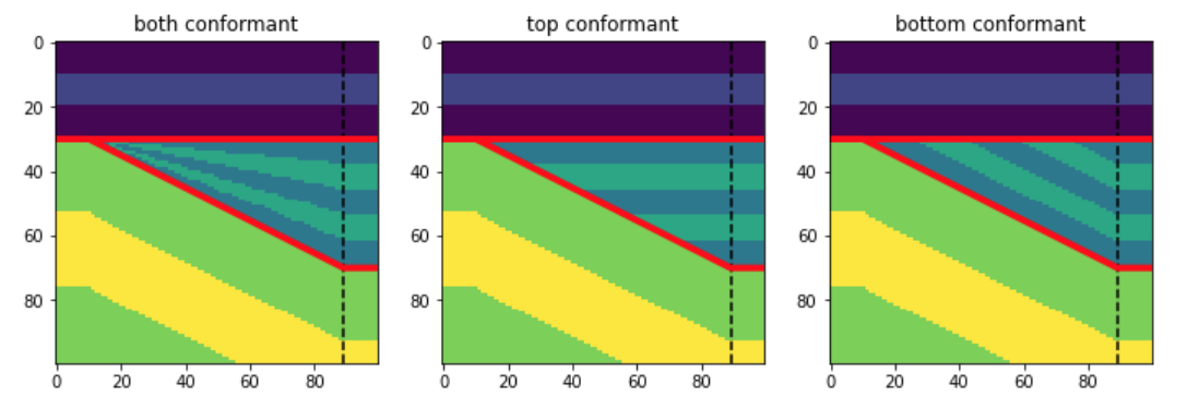
And here are some examples of what this will produce, depending on the conformance argument:

wedge_conformance.png

What’s new

I thought it might be interesting to be able to add another dimension to the wedge model — in and out of the screen in the models shown above. In that new dimension — as long as there are only two rock types in there — we could vary the “net:gross” of the wedge.

So if we have two rock types in the wedge, let’s say 2 and 3 as in the wedges shown above, we’ll end up with a lot of different wedges. At one end of the new dimension, we’ll have a wedge that is all 2. At the other end, it’ll be all 3. And in between, there’ll be a mixture of 2 and 3, with the layers interfingering in a geometrically symmetric way.

Let’s look at those 3 slices in the central model shown above:

bruges_wedge_slices.png

We can also see slices in that other dimension, to visualize the net:gross variance across the model. These slices are near the thin end of the wedge, the middle, and the thick end:

bruges_netgross_slices.png

To get 3D wedge models like this, just make a binary (2-component) wedge and add breadth=100 (the number of slices in the new dimension).

These models are admittedly a little mind-bending. Here’s what slices in all 3 orthogonal directions look like, along with (very badly) simulated seismic through this 3D wedge model:

bruges_all_the_slices.png

New wedge shapes!

As well as the net-to-gross thing, I added some new wedge shapes, so now you can have some steep-sided alternatives to the linear and sigmoidal ramps I had in there originally. In fact, you can pass in a wedge shape function of your own, so there’s no end to what you could implement.

bruges_new_wedge_shapes.png

You can read about these new features in this notebook. Please note that you will need the latest version of bruges to use these new features, so run pip install —upgrade bruges in your environment, then you’ll be all set. Share your models, I’d love to see what you make!

Survival of the fittest or overcrowding?

If you’ve been involved in drilling boreholes in your career, you’ll be familiar with desurvey. Desurvey is the process of converting a directional well survey — which provides measured depth, inclination and azimuth points from the borehole — into a position log. The position log is an arbitrarily finely sampled set of (x, y, z) points along the wellbore. We need this to convert from measured depth (distance along the borehole path) to depth in the earth, which is usually given relative to mean sea-level.

I hunted around recently and found no fewer than nine Python packages that contain desurvey code. They are of various vintages and licences:

Other larger tools that contain desurvey code but not as re-usable

This is amazing — look at all the activity in the last 2 years or so! I think this is a strong sign that we've hit a new era in geocomputing. Fifteen years ago a big chunk of the open source geoscience stuff out there was the ten-or-so seismic processing libraries. Then about 7 or 8 years ago there was a proliferation of geophysical modeling and inversion tools. Now perhaps we're seeing the geological and wells communities entering the same stage of evolution. This is encouraging.

What now?

But there’s a problem here too. — this is a small community, with limited resources. Can we afford this diversity? I accept that there might be a sort of Cambrian explosion event that has to happen with new technology. But how can we ensure that it results in an advantageous “survival of the fittest” ecology, and avoid it becoming just another way for the community to spread itself too thinly? To put it another way, how can we accelerate the evolutionary process, so that we don’t drain the ecosystem of valuable resources?

There’s also the problem of how to know which of these tools is the fittest. As far as I’m aware, there are no well trajectory benchmarks to compare against. Some of the libraries I listed above do not have rigorous tests, certainly they all have bugs (it’s software) — how can we ensure quality emerges from this amazing pool of technology?

I don’t know, but I think this is a soluble problem. We’ve done the hard part! Nine times :D


swung_round_135px.png

There was another sign of subsurface technology maturity in the TRANSFORM conference this year. Several of the tutorials and hackathon projects were focused on integrating tools like GemPy, Devito, segyio, and the lasio/welly/striplog family. This is exciting to see — 2021 could be an important year in the history of the open subsurface Python stack. Stay tuned!

All the wedges

Wedges are a staple of the seismic interpreter’s diet. These simple little models show at a glance how two seismic reflections interact with each other when a rock layer thins down to — and below — the resolution limit of the data. We can also easily study how the interaction changes as we vary the wavelet’s properties, especially its frequency content.

Here’s how to make and plot a basic wedge model with Python in the latest version of bruges, v0.4.2:

 
import bruges as bg
import matplotlib.pyplot as plt

wedge, *_ = bg.models.wedge()

plt.imshow(wedge)
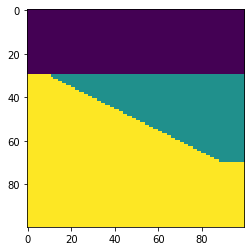
wedge_basic.png

It really is that simple! This model is rather simplistic though: it contains no stratigraphy, and the numerical content of the 2D array is just a bunch of integers. Let’s instead make a P-wave velocity model, with an internal bed of faster rock inside the wedge:

 
strat = [2.35, (2.40, 2.50, 2.40), 2.65]
wedge, *_ = bg.models.wedge(strat=strat)

plt.imshow(wedge)
plt.colorbar()
wedge_layer.png

We can also choose to make the internal geometry top- or bottom-conformant, mimicking onlap or an unconformity, respectively.

 
strat = strat=[0, 7*[1,2], 3]
wedge, *_ = bg.models.wedge(strat=strat,
                            conformance='base'
                           )

plt.imshow(wedge)
wedge_unconformity.png

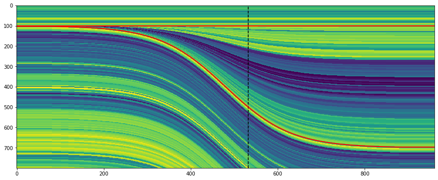
The killer feature of this new function might be using a log to make the stratigraphy, rather than just a few beds. This is straightforward to do with welly, because it makes selecting depth intervals and resampling a bit easier:

 
import welly

gr = welly.Well.from_las('R-39.las').data['GR']
log_above = gr.to_basis(stop=2620, step=1.0)
log_wedge = gr.to_basis(start=2620, stop=2720, step=1.0)
log_below = gr.to_basis(start=2720, step=1.0)

strat = (log_above, log_wedge, log_below)
depth, width = (100, 400, 100), (40, 200, 40)
wedge, top, base, ref = bg.models.wedge(depth=depth,
                                        width=width,
                                        strat=strat,
                                        thickness=(0, 1.5)
                                       )

plt.figure(figsize=(15, 6))
plt.imshow(wedge, aspect='auto')
plt.axvline(ref, color='k', ls='--')
plt.plot(top, 'r', lw=2)
plt.plot(base, 'r', lw=2)
wedge_log.png

Notice that the function returns to you the top and base of the wedgy part, as well as the position of the ‘reference’, in this case the well.

I’m not sure if anyone wanted this feature… but you can make clinoform models too:

wedge_log_clino.png

Lastly, the whole point of all this was to make a synthetic — the forward model of the seismic experiment. We can make a convolutional model with just a few more lines of code:

 
strat = np.array([2.32 * 2.65,  # Layer 1
                  2.35 * 2.60,  # Layer 2
                  2.35 * 2.62,  # Layer 3
                 ])

# Fancy indexing into the rocks with the model.
wedge, top, base, ref = bg.models.wedge(strat=strat)

# Make reflectivity.
rc = (wedge[1:] - wedge[:-1]) / (wedge[1:] + wedge[:-1])

# Get a wavelet.
ricker = bg.filters.ricker(0.064, 0.001, 40)

# Repeated 1D convolution for a synthetic.
syn = np.apply_along_axis(np.convolve, arr=rc, axis=0, v=ricker, mode='same')
wedge_synthetic.png

That covers most of what the tool can do — for now. I’m working on extending the models to three dimensions, so you will be able to vary layers or rock properties in the 3rd dimension. In the meantime, take these wedges for a spin and see what you can make! Do share your models on Twitter or LinkedIn, and have fun!

Future proof

Last week I wrote about the turmoil many subsurface professionals are experiencing today. There’s no advice that will work for everyone, but one thing that changed my life (ok, my career at least) was learning a programming language. Not only because programming computers is useful and fun, but also because of the technology insights it brings. Whether you’re into data management or machine learning, workflow automation or just being a more rounded professional, there really is no faster way to build digital muscles!

learn_python_thumb_2.png

Six classes

We have six public classes coming up in the next few weeks. But there are thousands of online and virtual classes you can take — what’s different about ours? Here’s what I think:

  • All of the instructors are geoscientists, and we have experience in sedimentology, geophysics, and structural geology. We’ve been programming in Python for years, but we remember how it felt to learn it for the first time.

  • We refer to subsurface data and typical workflows throughout the class. We don’t use abstract or unfamiliar examples. We focus 100% on scientific computing and data visualization. You can get a flavour of our material from the X Lines of Python blog series.

  • We want you to be self-sufficient, so we give you everything you need to start being productive right away. You’ll walk away with the full scientific Python stack on your computer, and dozens of notebooks showing you how to do all sorts of things from loading data to making a synthetic seismogram.

Let’s look at what we have on offer.

python_examples.png

Upcoming classes

We have a total of 6 public classes coming up, in two sets of three classes: one set with timing for North, Central and South America, and one set with timing for Europe, Africa, and the Middle East. Here they are:

  • Intro to Geocomputing, 5 half-days, 15–19 Feb — 🌎 Timing for Americas — 🌍 Timing for Europe & Africa — If you’re just getting started in scientific computing, or are coming to Python from another language, this is the class for you. No prerequisites.

  • Digital Geology with Python, 4 half-days, 22–25 Feb — 🌍 Timing for Europe & Africa — A closer look at geological workflows using Python. This class is for scientists and engineers with some Python experience.

  • Digital Geophysics with Python, 4 half-days, 22–25 Feb — 🌎 Timing for Americas — We get into some geophysical workflows using Python. This class is for quantitative scientists with some Python experience.

  • Machine Learning for Subsurface, 4 half-days in March — 🌎 Timing for Americas (1–4 Mar) — 🌍 Timing for Europe & Africa (8–11 Mar) — The best way into machine learning for earth scientists and subsurface engineers. We give you everything you need to manage your data and start exploring the world of data science and machine learning.

Follow the links above to find out more about each class. We have space for 14 people in each class. You find pricing options for students and those currently out of work. If you are in special circumstances, please get in touch — we don’t want price to be a barrier to these classes.

In-house options

If you have more than about 5 people to train, it might be worth thinking about an in-house class. That way, the class is full of colleagues learning things together — they can speak more openly and share more freely. We can also tailor the content and the examples to your needs more easily.

Get in touch if you want more info about this approach.

x lines of Python: static basemaps with contextily

Difficulty rating: Beginner

Something that is often useful in planning is to have a basemap of the area in which you have data or an interest. This can be made using a number of different tools, up to and including full-fledged GIS software, but we will use Contextily for a quick static basemap using Python. Installation is as simple as using conda install contextily or pip install contextily.

The steps that we want to take are the following, expressed in plain English, each of which will roughly be one line of code:

  1. Get a source for our basemap (placenames and similar things)
  2. Get a source for our geological map
  3. Get the location that we would like to map
  4. Plot the location with our geological data
  5. Add the basemap to our geological map
  6. Add the attribution for both maps
  7. Plot our final map

We will start with the imports, which as usual do not count:

 
import contextily as ctx
import matplotlib.pyplot as plt

Contextily has a number of built-in providers of map tiles, which can be accessed using the ctx.providers dictionary. This is nested, with some providers offering multiple tiles. An example is the ctx.providers.OpenStreetMap.Mapnik provider, which contains the following:

 
{'url': 'https://{s}.tile.openstreetmap.org/{z}/{x}/{y}.png',
 'max_zoom': 19,
 'attribution': '(C) OpenStreetMap contributors',
 'name': 'OpenStreetMap.Mapnik'}

The most important parameter in the dictionary for each provider is the url. These are of the form example.com/{z}/{x}/{y}.png. The {z} is the zoom level, while {x} and {y} relate to the latitude and longitude of a given tile, respectively. Note that these are the same as those used by interactive Slippy maps; contextily just downloads them as a single static image.

The easiest is to use one of these providers, but we can also define our own provider, using the above pattern for the URL. For geological data, the Macrostrat project is a great resource, especially because they have a tileserver supplying some detail. Their tileserver can be added using

 
geology_tiles = 'https://tiles.macrostrat.org/carto/{z}/{x}/{y}.png'

We also need a place to map. Contextily has a geocoder that can return the tiles covering a given location. It uses OpenStreetMap, so anything that is present there is useable as a location. This includes countries (e.g. 'Paraguay'), provinces/states ('Nova Scotia'), cities ('Lubumbashi'), and so on.

We will use Nova Scotia as our area of interest, as well as giving our desired map tiles. We can also use .plot() on the Place object to get a look at it immediately, using that basemap.

 
ctx.Place('Nova Scotia', source=ctx.providers.CartoDB.Positron).plot()
The Positron style from Carto for Nova Scotia.

The Positron style from Carto for Nova Scotia.

We'll use a different basemap though:

 
basemap = ctx.providers.Stamen.Toner

We can create the Place with our desired source — geology_tiles in this case — and then plot this on the basemap with some transparency. We will also add an attribution, since we need to credit MacroStrat.

 
place = ctx.Place('Nova Scotia', source=geology_tiles)

base_ax = place.plot()
ctx.add_basemap(ax=base_ax, source=basemap, alpha=0.5)
text = basemap.attribution + ' | Geological data: MacroStrat.org (CC-BY)'
ctx.add_attribution(ax=base_ax, text=text)

Finally, after a plt.show() call, we get the following:

nova_scotia_geology.png

Obviously this is still missing some important things, like a proper legend, but as a quick overview of what we can expect in a given area, it is a good approach. This workflow is probably better suited for general location maps.

Contextily also plays well with geopandas, allowing for an easy locality map of a given GeoDataFrame. Check out the accompanying Notebook for an example.

Binder  Run the accompanying notebook in MyBinder

Learn to code in 2020

Happy New Year! I hope 2020 is going well so far and that you have audacious plans for the new decade.

Perhaps among your plans is learning to code — or improving your skills, if you’re already on the way. As I wrote in 2011, programming is more than just writing code: it’s about learning a new way to think, not just about data but about problems. It’s also a great way to quickly raise your digital literacy — something most employers value more each year. And it’s fun.

We have three public courses planned for 2020. We’re also planning some public hackathons, which I’ll write about in the next week or three. Meanwhile, here’s the lowdown on the courses:

Lausanne in March

Rob Leckenby will be teaming up with Valentin Metraux of Geo2X to teach this 3-day class in Lausanne, Switzerland. We call it Intro to Geocomputing and it’s 100% suitable for beginners and people with less than a year or so of experience in Python. By the end, you’ll be able to read and write Python, write functions, read files, and run Jupyter Notebooks. More info here.

Amsterdam in June

If you can’t make it to Lausanne, we’ll be repeating the Intro to Geocomputing class in Amsterdam, right before the Software Underground’s Amstel Hack hackathon event (and then the EAGE meeting the following week). Check out the Software Underground Slack — look for the #amstel-hack-2020 channel — to find out more about the hackathon. More info here.

Houston in June

There’s also a chance to take the class in the US. The week before AAPG (which clashes with EAGE this year, which is very weird), we’ll be teaching not one but two classes: Intro to Geocomputing, and Intro to Machine Learning. You can take either one, or both — but be aware that the machine learning class assumes you know the basics of Python and NumPy. More info here.

In-house options

We still teach in-house courses (last year we taught 37 of them!). If you have more than about 5 people to train, then in-house is probably the way to go; we’d be delighted to work with you to figure out the best curriculum for your team.

Most of our classes fall into one of the following categories:

  • Beginner classes like the ones described above, usually 3 days.

  • Machine learning classes, like the Houston class above, usually 2 or 3 days.

  • Other more advanced classes built around engineering skills (object-oriented programming, testing, packaging, and so on), usually 3 days.

  • High-level digital literacy classes for middle to upper management, usually 1 day.

We also run hackathons and design sprints for teams that are trying to solve tricky problems in the digital subsurface, but those are another story…

Get in touch if you want more info about any of these.


Whatever you want to learn in 2020, give it everything you have. Schedule time for it. The discipline will pay off. If we can help or support you somehow, please let us know — above all, we want you to succeed.

Superpowers for striplogs

In between recent courses and hackathons, I’ve been chipping away at some new features in striplog. An open-source Python package, striplog handles irregularly sampled data, like lithologic intervals, chronostratigraphic zones, or anything that isn’t regularly sampled like, say, a well log. Instead of defining what is present at every depth location, you define intervals with a top and a base. The interval can contain whatever you like: names of rocks, images, or special core analyses, or anything at all.

You can read about all of the newer features in the changelog, but let’s look at a couple of the more interesting ones…

Binary morphology filters

Sometimes we’d like to simplify a striplog a bit, for example by ‘weeding out’ the thin beds. The tool has long had a method prune to systematically remove all intervals (e.g. beds) thinner than some cutoff; one can then optionally anneal the gaps, and merge the resulting striplog to combine similar neighbours. The result of this sequence of operations (prune, anneal, merge, or ‘PAM’) is shown below on the left.

striplog_binary_ops.png

If the intervals of a striplog have at least one property of a binary nature — with only two states, like sand and shale, or pay and non-pay — one can also use binary morphological operations. This well-known image processing technique aims to simplify data by eliminating small things. The result of opening vs closing operations is shown above.

Markov chains

I wrote about Markov chains earlier this year; they offer a way to identify bias in the order of units in a stratigraphic column. I’ve now put all the code into striplog — albeit not in a very fancy way. You can import the Markov_chain class from striplog.markov, then use it in exactly the same way as in the notebook I shared in that Markov chain post:

I started with some pseudorandom data (top) representing a known succession of Mudstone (M), Siltstone (S), Fine Sandstone (F) and coarse sandstone (C). Then I generate a Markov chain model of the succession. The chi-squared test indicates that the succession is highly unlikely to be unordered. We can look at the normalized difference matrix, generate a synthetic sequence of lithologies, or plot the difference matrix as a heatmap or a directed graph. The graph illustrates the order we originally imposed: M-S-F-C.

There is one additional feature compared to the original implementation: multi-step Markov chains. Previously, I was only looking at immediately adjacent intervals (beds or whatever). Now you can look at actual vs expected transition frequencies for next-but-one interval, or next-but-two. Don’t ask me how to interpret that information though…

Other new things

  • New ways to anneal. Now the user can choose whether the gaps in the log are filled in by flooding upwards (that is, by extending the interval below the gap upwards), flooding downwards (extending the upper interval), or flooding symmetrically into the middle from both above and below, meeting in the middle. (Note, you can also fill gaps with another component, using the fill() method.)

  • New merging strategies. Now you can merge overlapping intervals by precedence, rather than by blending the contents of the intervals. Precedence is defined however you like; for example, you can choose to keep the thickest interval in all overlaps, or if intervals have a date, you could keep the latest interval.

  • Improved bar charts. The histogram is easier to use, and there is a new bar chart summary of intervals. The bars can be sorted by any property you like.

Try it out and help add new stuff

You can install the latest version of striplog using pip. It’s as easy as:

pip install striplog

Start by checking out the tutorial notebooks in the repo, especially Striplog_basics.ipynb. Let me know how you get on, or jump on the Software Underground Slack to ask for help.

Here are some things I’d like striplog to support in the future:

  • Stratigraphic prediction.

  • Well-to-well correlation.

  • More interactions with well logs.

What ideas do you have? Or maybe you can help define how these things should work? Either way, do get in touch or check out the Striplog repository on GitHub.

x lines of Python: Loading images

Difficulty rating: Beginner

We'd often like to load images into Python. Once loaded, we might want to treat them as images, for example cropping them, saving in another format, or adjusting brightness and contrast. Or we might want to treat a greyscale image as a two-dimensional NumPy array, perhaps so that we can apply a custom filter, or because the image is actually seismic data.

This image-or-array duality is entirely semantic — there is really no difference between images and arrays. An image is a regular array of numbers, or, in the case of multi-channel rasters like full-colour images, a regular array of several numbers: one for each channel. So each pixel location in an RGB image contains 3 numbers:

raster_with_RGB_triples.png

In general, you can go one of two ways with images:

  1. Load the image using a library that 'knows about' (i.e. uses language related to) images. The preeminent tool here is pillow (which is a fork of the grandparent of all Python imaging solutions, PIL).
  2. Load the image using a library that knows about arrays, like matplotlib or scipy. These wrap PIL, making it a bit easier to use, but potentially losing some options on the way.

The Jupyter Notebook accompanying this post shows you how to do both of these things. I recommend learning to use some of PIL's power, but knowing about the easier options too.

Here's the way I generally load an image:

 
from PIL import Image
im = Image.open("my_image.png")

(One strange thing about pillow is that, while you install it with pip install pillow, you still actually import and use PIL in your code.) This im is an instance of PIL's Image class, which is a data structure especially for images. It has some handy methods, like im.crop(), im.rotate(), im.resize(), im.filter(), im.quantize(), and lots more. Doing some of these operations with NumPy arrays is fiddly — hence PIL's popularity.

But if you just want your image as a NumPy array:

 
import numpy as np
arr = np.array(im)

Note that arr is a 3-dimensional array, the dimensions being row, column, channel. You can go off with arr and do whatever you need, then cast back to an Image with Image.fromarray(arr).

All this stuff is demonstrated in the Notebook accompanying this post, or you can use one of these links to run it right now in your browser:

Binder   Run the accompanying notebook in MyBinder