Comparing regressors

There are several really nice comparisons between various algorithms in the Scikit-Learn documentation. The most famous, and useful, one is probably the classifier comparison:

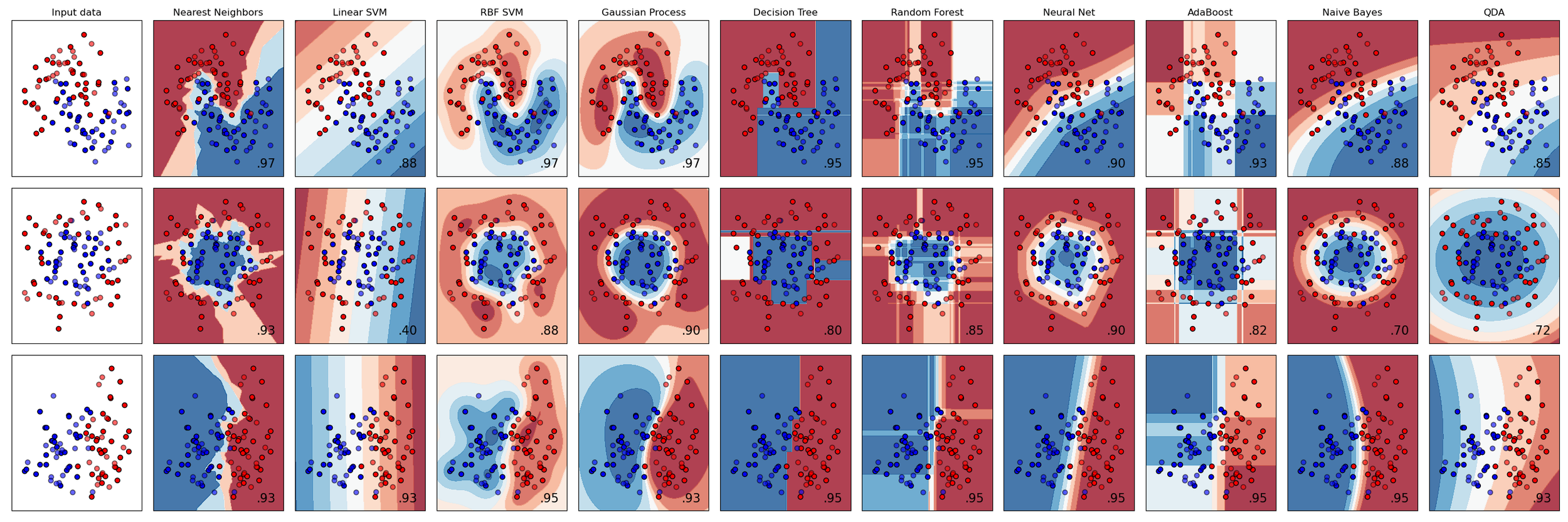
A comparison of classification algorithms. Each row is a different dataset; each column (except the first) is a different classifier, each trying to separate the blue and red points. The accuracy score of each classifier is show in the lower right corner of each plot. There’s so much to look at in this one plot!

There’s also a very nice clustering algorithm comparison, and this anomaly detection comparison. As usual with awesome open source software packages like Scikit-Learn, the really wonderful thing is that all the source code is right there so you can hack these things to show your own data.

What about regression?

Regression problems are the other major kind of machine learning task. If the thing you’re trying to predict is not a category (like ‘blue’ or ‘red’, as above) but a continuous property (like porosity, say), then you’re looking at a regression problem.

I wondered what a comparison plot for the various regressors in Scikit-Learn would look like. I couldn’t find one, so I made one. I made up three one-dimensional datasets — one linear, one polynomial, and one periodic. Then I tried predicting each one with various different model types, from linear regression to a deep neural network. Here’s version 1 (well, 0.1 really) of my script; feel free to adapt and improve it!

Here’s the plot it produces:

A comparison of most of the regressors in scikit-learn, made with this script. The red lines are unregularized models; the blue have regularization. The pale points are the validation data. The small numbers in each plot are RMS error (lower is better!).

I think this plot repays careful study. Notice the smoothing effect of regularization. See how tree-based methods result in discretized predictions, and kernel-based ones are pretty horrible at extrapolation.

I’m 100% open to feedback on ways to improve this plot… or please improve it and show me how it goes!

The procedural generation of geology

Procedural generation is a way of faking stuff with computers. But by writing code, or otherwise defining algorithms — not by manually choosing or composing or sculpting things. It’s used to produce landscapes and other assets in computer games, or just to make beautiful things. Honestly, I know almost nothing about it, and I don’t play computer games, so I’m really just coming at it from the ‘beautiful things’ side. So let’s just stick to looking at some examples…

Robert Hodgin produces jaw-dropping images, and happily one of his favourite subjects is meandering rivers. Better yet, Harold Fisk’s maps are among his inspirations. The results are mindblowing — just check this animation out:

What’s really remarkable is that everything on that map is procedurally generated: the roadways, the vegetation, the wonderful names.

If you love meanders (who doesn’t love meanders?), then you also need to know about Zoltan Sylvester’s work (not to mention his Etsy store). He produces some great animations, and also maintains some open-source Python projects (e.g. meanderpy) for producing them, so you can get stuck in and make your own.

It’s not just about meanders. Artist Tyler Hobbs has produced some striking images that strongly resemble structural cross-sections. In this thread he mentions that this wasn’t his goal, they just came out that way.

Mattias Herder, a space-obsessed viz wizard, did intend to produce crystals though. He’s using Houdini software, which I believe is also what Robert Hodgin uses for his maps. I wonder if any geologists are using it…

Landscapes are one of the big areas of application of this sort of tech, and while not strictly geological, I love these frozen vistas by French artist Guillaume Cottet:

Finally, this example from digital artist Ian Smith hints at a bit of the creative process. This guy really knows how to make rocks…

This is all so much magic to me, but I’m intrigued. Like the black hole in Interstellar, could this kind of work actually shed light on how dynamic, non-linear natural systems work? Or is it just an illusion?

Illuminated equations

Last year I wrote a post about annotated equations, and why they are useful teaching tools. But I never shared all the cool examples people tweeted back, and some of them are too good not to share.

Let’s start with this one from Andrew Alexander that he uses to explain complex number notation:

illuminated_complex.png

Paige Bailey tweeted some examples of annotated equations and code from the reinforcement learning tutorial, Building a Powerful DQN in TensorFlow by Sebastian Theiler. Here’s one of the algorithms, with slightly muted annotations:

Illuminated_code_Theiler_edit.jpeg.png

Finally, Jesper Dramsch shared a new one today (and reminded me that I never finished this post). It links to Edward Raff’s book, Inside Deep Learning, which has some nice annotations, e.g. expressing a fundamental idea of machine learning:

Raff_cost_function.png

Dynamic explication

The annotations are nice, but it’s quite hard to fully explain an equation or algorithm in one shot like this. It’s easier to do, and easier to digest, over time, in a presentation. I remember a wonderful presentation by Ross Mitchell (then U of Calgary) at the also brilliant lunchtime mathematics lectures that Shell used to sponsor in Calgary. He unpeeled time-frequency analysis, especially the S transform, and I still think about his talk today.

What Ross understood is that the learner really wants to see the maths build, more or less from first principles. Here’s a nice example — admittedly in the non-ideal medium of Twitter: make sure you read the whole thread — from Darrel Francis, a cardiologist at Imperial Colege, London:

A video is even more dynamic of course. Josef Murad shared a video in which he derives the Navier–Stokes equation:

In this video, Grant Sanderson, perhaps the equation explainer nonpareil, unpacks the Fourier transform. He creeps up on the equation, starting instead with building the intuition around frequency decomposition:

If you’d like to try making this sort of thing, you might like to know that Sanderson’s Python software, manim, is open source.


Multi-modal explication

Sanderson illustrates nicely that the teacher has several pedagogic tools at their disposal:

  • The spoken word.

  • The written word, especially the paragraph describing a function.

  • A symbolic representation of the function.

  • A graphical representation of the function.

  • A code representation of the function, which might also have a docstring, which is a formal description of the code, its inputs, and its outputs. It might also produce the graphical representation.

  • Still other modes, e.g. pseudocode (see Theiler’s example, above), a cartoon (esssentially a ‘pseudofigure’),

Virtually all of these things are, or can be dynamic (in a video, on a whiteboard) and annotated. They approach the problem from different directions. The spoken and written descriptions should be rigorous and unambiguous, but this can make them clumsy. Symbolic maths can be useful to those that can read it, but authors must take care to define symbols properly and to be consistent. The code representation must be strict (assuming it works), but might be hard for non-programmers to parse. Figures help most people, but are more about building intuition than providing the detail you might need for implementation, say. So perhaps the best explanations have several modes of explication.

In this vein of multi-modal explication, Jeremy Howard shared a nice example from his book, Deep learning for coders, of combining text, symbolic maths, and code:

illuminated_jeremy_howard.png

Eventually I settled on calling these things, that go beyond mere annotation, illuminated equations (not to directly compare them to the beautiful works of devotion produced by monks in the 13th century, but that’s the general idea). I made an attempt to describe linear regression and the neural network equation (not sure what else to call it!) in a series of tweets last year. Here’s the all-in-one poster version (as a PDF):

linear_inversion_page.png

There’s nothing intuitive about physics, maths, or programming. The more tricks we have for spreading intuition about these important scientific tools, the better. I think there’s something in illuminated equations for teachers to practice — and students too. In fact, Jackie Caplan-Auerbach decribes coaching her students in creating ‘equation dictionaries’ in her geophysics classes. I think this is a wonderful idea.

If you’re teaching or learning maths, I’d love to hear your thoughts. Are these things worth the effort to produce? Do you have any favourite examples to share?

x lines of Python: Stereonets

Difficulty rating: Intermediate

A few years back I needed to plot some fracture data without specialist software, so I created an Excel spreadsheet with a polar plot and interactive widgets. But thanks to Joe Kington and his awesome mplstereonet library those days are over. Today I want to share with you how to plot two fracture sets on an equal area Schmidt plot with mplstereonet.

Here's what we're going to do — and in only 10 lines of Python:

  1. Load the data from a CSV file.
  2. Create a stereonet with grid lines.
  3. Loop over fracture sets and plot each in a different colour.
  4. Add some statistics for each set.

For data we'll use Irene Wallis's fantastic open-source project fractoolbox repo, which includes some data — as well as some notebooks that go beyond what we will do here.

This results in the plot shown here, where each fracture is plotted as a point representing the pole of the fracture plane.

We see that not counting the imports, we can make this simple plot with as a few as 10 lines of code while still retaining some flexibility to refactor this code. The accompanying notebook also shows how to use ipywidgets to make the plot interactive.

stereonet_example.jpg

That’s it! There’s more in the Notebook — check out the links below. If you get some beautiful plots out of your data, share them in the Software Underground or on Twitter. Have fun!

GitHub    See the Notebook on GitHub

Binder    Run the Notebook in MyBinder

Visual explanations of mathematics

It is thought that Euclid wrote Elements in about 300 BC, but Oliver Byrne turned it into one of the true gems of visualization — and made it about 100 times more readable. By seamlessly combining typeset text (Caslon, if you’re interested) with minimalist geometric drawings in primary colours, he didn’t just reproduce the text; he explained it in a new way.

annotated_byrne_euclid.png

If you like the look of it, it’s even cooler in Nicholas Rougeur’s beautiful interactive version.

This is a classic example of what Edward Tufte, the modern saint of visualization, calls a visual explanation (he wrote a whole book about the subject). We’ve written about the subject before (for example, see Evan’s 2014 post, Graphics that repay careful study). Figures and charts should do more than merely illustrate, they should elucidate.

Too often, equations — for example the myriad equations in any volume of GEOPHYSICS — do not elucidate. Indeed, they barely even illustrate. In some cases, it’s worse: they obfuscate. You might think mathematics is too dry, or too steeped in convention, for it to be any other way. Equations just are. But Byrne showed us that we can do better.

A few years ago, in an attempt to broaden my geophysical knowledge, I bought a copy of Daniel Fleisch’s book on Maxwell’s equations. It’s excellent, and the others in the series are good too. I especially liked the annotated equations; I’ve lightened the annotations in this version, to put them on a separate visual ‘layer’:

annotated_maxwell_by_fleisch.jpeg

In 2010, Randall Munroe of xkcd applied a similar strategy to label The Flake Equation, his parody of the Drake equation:

annotated_flake_equation.png

There are still other examples out there.

Later, I came across some lovely colourized equations by Stuart Riffle, a game developer. There was a bit of buzz about them on social media. Most people loved them, but a few pointed out that they suffer from the ‘legend lookup’ problem, and the colours he chose might not be great for colourblind people. Still, I like the concept — here’s the Fourier transform:

annotated_Fourier_Transform.png

Direct annotation, something Tufte always advocates, avoids the legend lookup problem. In his 2016 Geophysics Tutorial on finite volume methods, Rowan Cockett showed that colour and labels can work together:

annotated_equation_by_rowan_cockett.jpeg

And in his Observable post on the predator–prey interaction, modern visualization legend Mike Bostock avoids the problem entirely with the use of pictograms: direct representation of what the symbols represent:

annotated_predator_prey.png

Observable is interesting because the documents are runnable code. And this reminds us that mathematics — equations, data structures, and so on — has another expression: code. While symbolic representation speaks directly to some people, code speaks to others, probably more. Look at Randall Munroe’s annotation of a Wolfram Alpha equation (similar to an Excel formula) from his (wonderful) book, What If:

annotated_golf_xkcd.png

What I love about this is the direct path to exploring the function yourself. It would take me an hour to implement Fleisch’s electric field integral in code, even with the annotations. Typing in this — admittedly less useful — rocket golf equation will take me two minutes. Expressing mathematics in code is the ultimate explicit and practical expression of an idea.

We have lots of tools to write better mathematics: LaTeX, markdown, Jupyter Notebooks, and so on. But it feels like nothing has really converged yet. Technology that seamlessly mixes symbolic equations, illustrative-and-explicative annotation, and runnable code is, I am sure, not far off. Until then, we do the best we can with the tools we have.


Have you seen nice examples of annotated equations? I’d love to hear about them; let me know in the comments!


Don’t miss the follow-up post from 2021: Illuminated equations.


The work by Byrne is out of copyright. Those by Munroe and Cockett are openly licensed under Creative Commons. The work of Fleisch and Bostock are used in accordance with Fair Use doctrine.

x lines of Python: Ternary diagrams

Difficulty rating: beginner-friendly

(I just realized that calling the more approachable tutorials ‘easy’ is perhaps not the most sympathetic way to put it. But I think this one is fairly approachable.)

If you’re new to Python, plotting is a great way to get used to data structures, and even syntax, because you get immediate visual feedback. Plots are just fun.

Data loading

The first thing is to load the data, which is contained in a Google Sheets spreadsheet. If you make a sheet public, it’s easy to make a URL that provides a CSV. Happily, the Python data management library pandas can read URLs directly, so loading the data is quite easy — the only slightly ugly thing is the long URL:

    import pandas as pd
    uid = "1r7AYOFEw9RgU0QaagxkHuECvfoegQWp9spQtMV8XJGI"
    url = f"https://docs.google.com/spreadsheets/d/{uid}/export?format=csv"
    df = pd.read_csv(url) 

This dataset contains results from point-counting 51 shallow marine sandstones from the Eocene Sobrarbe Formation. We’re going to plot normalized volume percentages of quartz grains, detrital carbonate grains, and undifferentiated matrix. Three parameters? Two degrees of freedom? Let’s make a ternary plot!

Data exploration

Once you have the data in pandas, and before getting to the triangular stuff, we should have a look at it. Seaborn, a popular statistical plotting library, has a nifty ‘pairplot’ which plots the numerical parameters against each other to help reveal patterns in the data. On the diagonal, it shows kernel density estimations to reveal the distribution of each property:

    import seaborn as sns
    vars = ['Matrix', 'Quartz', 'Carbonate', 'Bioclasts', 'Authigenic']
    sns.pairplot(df, vars=vars, hue='Facies Association')
ternary_data_pairplot.png

Normalization is fairly straightforward. For each column, e.g. df['Carbonate'], we make a new column, e.g. df['C'], which is normalized to the sum of the three components, given by df[cols].sum(axis=1):

cols = ['Carbonate', 'Quartz', 'Matrix']
for col in cols:
    df[col[0]] = df[col] * 100 / df[cols].sum(axis=1)

The ternary plot

For the ternary plot itself I’m using the python-ternary library, which is pretty hands-on in that most plots take quite a bit of code. But the upside of this is that you can do almost anything you want. (Theres one other option for Python, the ever-reliable plotly, and there’s a solid-looking package for R too in ggtern.)

We just need a few lines of plotting code (left) to pull a ternary diagram (right) together.

    fig, tax = ternary.figure(scale=100)
    fig.set_size_inches(5, 4.5)

    tax.scatter(df[['M', 'Q', 'C']].values)
    tax.gridlines(multiple=20)
    tax.get_axes().axis('off')
ternary_tiny.png

But here you see what I mean about this being quite a low-level library: each element of the plot has to be added explicitly. So if we want axis labels, titles, and other annotations, we need more code… all of which is laid out in the accompanying notebook. You can download this from GitHub, or run it right now, right in your browser, with these links:

Binder   Run the accompanying notebook in MyBinder

Open In Colab   Run the notebook in Google Colaboratory (note you need to install python-ternary)

Give it a go, and have fun making your own ternary plots in Python! Share them on LinkedIn or Twitter.

Quartz, carbonate and matrix quantities (normalized to 100%) for 51 calcareous sandstones from the Eocene Sobrarbe Formation. The ternary plot was made with python-ternary library for Python and matplotlib.

Quartz, carbonate and matrix quantities (normalized to 100%) for 51 calcareous sandstones from the Eocene Sobrarbe Formation. The ternary plot was made with python-ternary library for Python and matplotlib.

Visualization in Copenhagen, part 2

In Part 1, I wrote about six of the projects teams contributed at the Subsurface Hackathon in Copenhagen in June. Today I want to tell you about the rest of them. 


A data exploration tool

Team GeoClusterFu...n: Dan Stanton (University of Leeds), Filippo Broggini (ETH Zürich), Francois Bonneau (Nancy), Danny Javier Tapiero Luna (Equinor), Sabyasachi Dash (Cairn India), Nnanna Ijioma (geophysicist). 

Tech: Plotly Dash. GitHub repo.

Project: The team set out to build an interactive web app — a totally new thing for all of them — to make interactive plots from data in a CSV. They ended up with the basis of a useful tool for exploring geoscience data. Project page.

Four sixths of the GeoClusterFu...n team cluster around a laptop.

Four sixths of the GeoClusterFu...n team cluster around a laptop.


AR outcrop on your phone

Team SmARt_OGs: Brian Burnham (University of Aberdeen), Tala Maria Aabø (Natural History Museum of Denmark), Björn Wieczoreck, Georg Semmler and Johannes Camin (GiGa Infosystems).

Tech: ARKit/ARCore, WebAR, Firebase. GitLab repo. 

Project: Bjørn and his colleagues from GiGa Infosystems have been at all the European hackathons. This time, he knew he wanted to get virtual outcrops on mobiles phones. He found a willing team, and they got it done! Project page.

Three views from the SmartOGs's video. See the full version.

Three views from the SmartOGs's video. See the full version.


Rock clusters in latent space

The Embedders: Lukas Mosser (Imperial College London), Jesper Dramsch (Technical University of Denmark), Ben Fischer (PricewaterhouseCoopers), Harry McHugh (DUG), Shubhodip Konar (Cairn India), Song Hou (CGG), Peter Bormann (ConocoPhillips).

Tech: Bokeh, scikit-learn, Multicore-TSNE. GitHub repo.

Project: There has been a lot of recent interest in the t-SNE algorithm as a way to reduce the dimensionality of complex data. The team explored its application to subsurface data, and found promising applications. Web page. Project page.

The Embeders built a web app to cluster the data in an LAS file. The clusters (top left) are generated by the t-SNE algorithm.

The Embeders built a web app to cluster the data in an LAS file. The clusters (top left) are generated by the t-SNE algorithm.


Fully mixed reality

Team Hands On GeoLabs: Will Sanger (Western Geco), Chance Sanger (Houston Museum of Fine Arts), Pierre Goutorbe (Total), Fernando Villanueva (Institut de Physique du Globe de Paris).

Project: Starting with the ambitious goal of combining the mixed reality of the Meta AR gear with the mixed reality of the Gempy sandbox, the team managed to display and interact with some seismic data in the AR headset, which  allows interaction with simple hand gestures. Project page.

The team demonstrate the Meta AR headset.

The team demonstrate the Meta AR headset.


Huge grids over the web

Team Grid Vizards: Fabian Kampe, Daniel Buse, Jonas Kopcsek, Paul Gabriel (all from GiGa Infosystems)

Tech: three.js. GitHub repo.

Project: Paul and his team wanted to visualize hundreds of millions or billions of grid cells — all in the browser. They ended up with about 20 million points working very smoothly, and impressed everyone. Project page.

grid_vizards.png

Interpreting RGB displays for spec decomp

Team: Florian Smit (Technical University of Denmark), Gijs Straathof (SGS), Thomas Gazzola (Total), Julien Capgras (Total), Steve Purves (Euclidity), Tom Sandison (Shell)

Tech: Python, react.js. GitHub repos: Client. Backend.

Project: Spectral decomposition is still a mostly quantitative tool, especially the interpretation of RGB-blended displays. This team set out to make intuitive, attractive forward models of the spectral response of wells. This should help interpret seismic data, and perhaps make more useful RGB displays too. Intriguing and promising work. Project page.

RGB_log.png

That's it for another year! Twelve new geoscience visualization projects — ten of them open source. And another fun, creative weekend for 63 geoscientists — all of whom left with new connections and new skills. All this compressed into one weekend. If you haven't experienced a hackathon yet, I urge you to seek one out.

I will leave you with two videos — and an apology. We are so focused on creating a memorable experience for everyone in the room, that we tend to neglect the importance of capturing what's happening. Early hackathons only had the resulting blog post as the document of record, but lately we've been trying to livestream the demos at the end. Our success has been, er, mixed... but they were especially wonky this time because we didn't have livestream maestro Gram Ganssle there. So, these videos exist, and are part of the documentation of the event, but they barely begin to convey the awesomeness of the individuals, the teams, or their projects. Enjoy them, but next time — you should be there!

Visualization in Copenhagen, part 1

CPH_blog_banner.png

It's finally here! The round-up of projects from the Subsurface Hacakthon in Copenhagen last month. This is the first of two posts presenting the teams and their efforts, in the same random order the teams presented them at the end of the event.


Subsurface data meets Pokemon Go

Team Geo Go: Karine Schmidt, Max Gribner, Hans Sturm (all from Wintershall), Stine Lærke Andersen (University of Copenhagen), Ole Johan Hornenes (University of Bergen), Per Fjellheim (Emerson), Arne Kjetil Andersen (Emerson), Keith Armstrong (Dell EMC). 

Project: With Pokemon Go as inspiration, the team set out to prototype a geoscience visualization app that placed interactive subsurface data elements into a realistic 3D environment.

180610_agile_scientific_78.jpg

Visualizing blind spots in data

Team Blind Spots: Jo Bagguley (UK Oil & Gas Authority), Duncan Irving (Teradata), Laura Froelich (Teradata), Christian Hirsch (Aalborg University), Sean Walker (Campbell & Walker Geophysics).

Tech: Flask, Bokeh, AWS for hosting app. GitHub repo.

Project: Data management always comes up as an issue in conversations about geocomputing, but few are bold enough to tackle it head on. This team built components for checking the integrity of large amounts of raw data, before passing it to data science projects. Project page.

Sean, Laura, and Christian. Jo and Duncan were out doing research. Note the kanban board in the background — agile all the way!

Sean, Laura, and Christian. Jo and Duncan were out doing research. Note the kanban board in the background — agile all the way!


Volume uncertainties visualization

Team Fortuna: Natalia Shchukina (Total), Behrooz Bashokooh (Shell), Tobias Staal (University of Tasmania), Robert Leckenby (now Agile!), Graham Brew (Dynamic Graphics), Marco van Veen (RWTH Aachen). 

Tech: Flask, Bokeh, Altair, Holoviews. GitHub repo.

Project: Natalia brought some data with her: lots of surface grids. The team built a web app to compute uncertainty sections and maps, then display them dynamically and interactively — eliciting audible gasps from the room. Project page.

The Fortuna app: Probability of being the the zone (left) and entropy (right). Cross-sections are shown at the top, maps on the bottom.


Differences and similarities with RGB blends

Team RGBlend: Melanie Plainchault and Jonathan Gallon (Total), Per Olav Svendsen, Jørgen Kvalsvik and Max Schuberth (Equinor).

Tech: Python, Bokeh. GitHub repo.

Project: One of the more intriguing ideas of the hackathon was not just so much a fancy visualization technique, as a novel way of producing a visualization — differencing 3 images and visualizing the differences in RGB space. It reminded me of an old blog post about the spot the difference game. Project page.

The differences (lower right) between three time-lapse seismic amplitude maps.

The differences (lower right) between three time-lapse seismic amplitude maps.


Augmented reality geological maps

Team AR Sandbox: Simon Virgo (RWTH Aachen), Miguel de la Varga (RWTH Aachen), Fabian Antonio Stamm (RWTH Aachen), Alexander Schaaf (University of Aberdeen).

Tech: Gempy. GitHub repo.

Project: I don't have favourite projects, but if I did, this would be it. The GemPy group had already built their sandbox when they arrived, but they extended it during the hackathon. Wonderful stuff. Project page.

magic box of sand: Sculpting a landscape (left), and the projected map (right). You can't even imagine how much fun it was to play with.


Augmented reality seismic wavefields

Team Sandbox Seismics: Yuriy Ivanov (NTNU Trondheim), Ana Lim (NTNU Trondheim), Anton Kühl (University of Copenhagen), Jean Philippe Montel (Total).

Tech: GemPy, Devito. GitHub repo.

Project: This team worked closely with Team AR Sandbox, but took it in a different direction. They instead read the velocity from the surface of the sand, then used devito to simulate a seismic wavefield propagating across the model, and projected that wavefield onto the sand. See it in action in my recent Code Show post. Project page.

Yuriy Ivanov demoing the seismic wavefield moving across the sandbox.


Pretty cool, right? As usual, all of these projects were built during the hackathon weekend, almost exclusively by teams that formed spontaneously at the event itself (I think one team was self-contained from the start). If you didn't notice the affiliations of the participants — go back and check them out; I think this might have been an unprecedented level of collaboration!

Next time we'll look at the other six projects. [UPDATE: Next post is here.]

Before you go, check out this awesome video Wintershall made about the event. A massive thank you to them for supporting the event and for recording this beautiful footage — and for agreeing to share it under a CC-BY license. Amazing stuff!

Visualize this!

The Copenhagen edition of the Subsurface Hackathon is over! For three days during the warmest June in Denmark for over 100 years, 63 geoscientists and programmers cooked up hot code in the Rainmaking Loft, one of the coolest, and warmest, coworking spaces you've ever seen. As always, every one of the participants brought their A game, and the weekend flew by in a blur of creativity, coffee, and collaboration. And croissants.

Pierre enjoying the Meta AR headset that DEll EMC provided.

Pierre enjoying the Meta AR headset that DEll EMC provided.

Our sponsors have always been unusually helpful and inspiring, pushing us to get more audacious, but this year they were exceptionally engaged and proactive. Dell EMC, in the form of David and Keith, provided some fantastic tech for the teams to explore; Total supported Agile throughout the organization phase, and Wintershall kindly arranged for the event to be captured on film — something I hope to be able to share soon. See below for the full credit roll!

sponsors.png

During th event, twelve teams dug into the theme of visualization and interaction. As in Houston last September, we started the event on Friday evening, after the Bootcamp (a full day of informal training). We have a bit of process to form the teams, and it usually takes a couple of hours. But with plenty of pizza and beer for fuel, the evening flew by. After that, it was two whole days of coding, followed by demos from all of the teams and a few prizes. Check out some of the pictures:

Thank you very much to everyone that helped make this event happen! Truly a cast of thousands:

  • David Holmes of Dell EMC for unparallelled awesomeness.
  • The whole Total team, but especially Frederic Broust, Sophie Segura, Yannick Pion, and Laurent Baduel...
  • ...and also Arnaud Rodde for helping with the judging.
  • The Wintershall team, especially Andreas Beha, who also acted as a judge.
  • Brendon Hall of Enthought for sponsoring the event.
  • Carlos Castro and Kim Saabye Pedersen of Amazon AWS.
  • Mathias Hummel and Mahendra Roopa of NVIDIA.
  • Eirik Larsen of Earth Science Analytics for sponsoring the event and helping with the judging.
  • Duncan Irving of Teradata for sponsoring, and sorting out the T-shirts.
  • Monica Beech of Ikon Science for participating in the judging.
  • Matthias Hartung of Target for acting as a judge again.
  • Oliver Ranneries, plus Nina and Eva of Rainmaking Loft.
  • Christopher Backholm for taking such great photographs.

Finally, some statistics from the event:

  • 63 participants, including 8 women (still way too few, but 100% better than 4 out of 63 in Paris)
  • 15 students plus a handful of post-docs.
  • 19 people from petroleum companies.
  • 20 people from service and technology companies, including 7 from GiGa-infosystems!
  • 1 no-show, which I think is a new record.

I will write a summary of all the projects in a couple of weeks when I've caught my breath. In the meantime, you can read a bit about them on our new events portal. We'll be steadily improving this new tool over the coming weeks and months.

That's it for another year... except we'll be back in Europe before the end of the year. There's the FORCE Hackathon in Stavanger in September, then in November we'll be in Aberdeen and London running some events with the Oil and Gas Authority. If you want some machine learning fun, or are looking for a new challenge, please come along!

Simon Virgo (centre) and his colleagues in Aachen built an augmented reality sandbox, powered by their research group's software, Gempy. He brought it along and three teams attempted projects based on the technology. Above, some of the participants …

Simon Virgo (centre) and his colleagues in Aachen built an augmented reality sandbox, powered by their research group's software, Gempy. He brought it along and three teams attempted projects based on the technology. Above, some of the participants are having a scrum meeting to keep their project on track.


Looking forward to Copenhagen

We're in Copenhagen for the Subsurface Bootcamp and Hackathon, which start today, and the EAGE Annual Conference and Exhibition, which starts next week. Walking around the city yesterday, basking in warm sunshine and surrounded by sun-giddy Scandinavians, it became clear that Copenhagen is a pretty special place, where northern Europe and southern Europe seem to have equal influence.

The event this weekend promises to be the biggest hackathon yet. It's our 10th, so I think we have the format figured out. But it's only the third in Europe, the theme — Visualization and interaction — is new for us, and most of the participants are new to hackathons so there's still the thrill of the unknown! 

Many thanks to our sponsors for helping to make this latest event happen! Support these organizations: they know how to accelerate innovation in our industry.

sponsors.png

New events for UK

By the way, we just announced two new hackathons, one in London and one in Aberdeen, for the autumn. They are happening just before PETEX, the PESGB petroleum conference; find out more here. You can skill up for these events at some new courses, also just announced. The UK Oil and Gas Authority is offering our Intro to Geocomputing and Machine Learning class for free — apply here for a place. The courses are oversubscribed, so be sure to tell the OGA why you should get a place!

Code Show

There is a lot of other stuff happening at the EAGE exhibition this year — the HPC area, a new start-up area, and a digital transformation area which I hope is as bold as it sounds. Here's the complete schedule and some highlights:

There's lots of other stuff of course — EAGE has the most varied programme of any subsurface conference — but these are the sessions I'd be at if I had time to go to any sessions this year. But I won't because The hackathon is not all that's happening! Next week, starting on Tuesday, we're conducting a new experiment with the Code Show. In partnership with EAGE and Total, this is our attempt to bring some of the hackathon experience to everyone at EAGE. We'll be showing people the projects from the hackathon, talking to them about programming, and helping them get started on their own coding adventure. So if you're at EAGE, swing by Booth #1830 and say Hi.