Reliable predictions of unlikely geology

A puzzle

Imagine you are working in a newly-accessible and under-explored area of an otherwise mature basin. Statistics show that on average 10% of structures are filled with gas; the rest are dry. Fortunately, you have some seismic analysis technology that allows you to predict the presence of gas with 80% reliability. In other words, four out of five gas-filled structures test positive with the technique, and when it is applied to water-filled structures, it gives a negative result four times out of five.

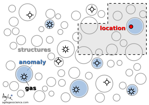
← It is thought that 10% of the structures in this play are gas-filled. Your seismic attribute test is thought to be 80% reliable, because four out of five times it has indicated gas correctly. You acquire the undrilled acreage shown by the grey polygon.

You acquire some undrilled acreage—the grey polygon— then delineate some structures and perform the analysis. One of the structures tests positive. If this is the only information you have, what is the probability that it is gas-filled?

This is a classic problem of embracing Bayesian likelihood and ignoring your built-in 'representativeness heuristic' (Kahneman et al, 1982, Judgment Under Uncertainty: Heuristics and Biases, Cambridge University Press). Bayesian probability combination does not come very naturally to most people but, once understood, can at least help you see the way to approach similar problems in the future. The way the problem is framed here, it is identical to the original formulation of Kahneman et al, the Taxicab Problem. This takes place in a town with 90 yellow cabs and 10 blue ones. A taxi is involved in a hit-and-run, witnessed by a passer-by. Eye witness reliability is shown to be 80%, so if the witness says the taxi was blue, what is the probability that the cab was indeed blue? Most people go with 80%, but in fact the witness is probably wrong. To see why, let's go back to the exploration problem and look at 100 test cases.

Break it down

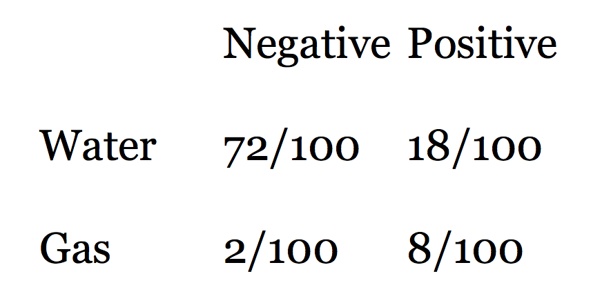Looking at the rows in this table of outcomes, we see that there are 90 water cases and 10 gas cases. Eighty percent of the water cases test negative, and 80% of the gas cases test positive. The table shows that when we get a positive test, the probability that the test is true is not 0.80, but much less: 8/(8+18) = 0.31. In other words, a test that is mostly reliable is probably wrong when applied to an event that doesn't happen very often (a structure being gas charged). It's still good news for us, though, because a probability of discovery of 0.31 is much better than the 0.10 that we started with.

Here is Bayes' Theorem for calculating the probability P of event A (say, a gas discovery) given event B (say, a positive test in our seismic analysis):

So we can express our problem in these terms:

Are you sure about that?

This result is so counter-intuitive, for me at least, that I can't resist illustrating it with another well-known example that takes it to extremes. Imagine you test positive for a very rare disease, seismitis. The test is 99% reliable. But the disease affects only 1 person in 10 000. What is the probability that you do indeed have seismitis?

Notice that the unreliability (1%) of the test is much greater than the rate of occurrence of the disease (0.01%). This is a red flag. It's not hard to see that there will be many false positives: only 1 person in 10 000 are ill, and that person tests positive 99% of the time (almost always). The problem is that 1% of the 9 999 healthy people, 100 people, will test positive too. So for every 10 000 people tested, 101 test positive even though only 1 is ill. So the probability of being ill, given a positive test, is only about 1/101!

Lessons learned

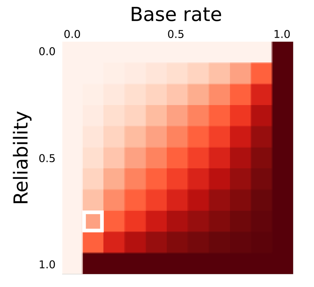← Predictive power (in Bayesian jargon, the posterior probability) as a function of test reliability and the base rate of occurrence (also called the prior probability of the event of phenomenon in question). The position of the scenario in the exploration problem is shown by the white square.

Thanks to UBC Bioinformatics for the heatmap software, heatmap.notlong.com.

Next time you confidently predict something with a seismic attribute, stop to think not only about the reliability of the test you have made, but the rate of occurrence of the thing you're trying to predict. The heatmap shows how prediction power depends on both test reliability and the occurrence rate of the event. You may be doing worse (or better!) than you think.

Fortunately, in most real cases, there is a simple mitigation: use other, independent, methods of prediction. Mutually uncorrelated seismic attributes, well data, engineering test results, if applied diligently, can improve the odds of a correct prediction. But computing the posterior probability of event A given independent observations B, C, D, E, and F, is beyond the scope of this article (not to mention this author!).

This post is a version of part of my article The rational geoscientist, The Leading Edge, May 2010

Update on 2011-07-12 23:31 by Matt Hall

Just flicking through the archives and came across this post about unlikely events and Bayes' theorem. I can't believe I forgot to link to it in this story. So I'm doing it now!

News of the week

CCGVeritas moves towards a million channels

Sercel, a subsidiary of CGGVeritas, has introduced new data transmission technology, Giga Transverse, an add-on to the 428XL land acquisition system. The technology increases the maximum channels per line from 10 000 to 100 000, and brings them a big step closer to the possiblity of one million channels on a single job. It will immediately benefit their UltraSeis offering for high-density point-receiver land acquisition. They also refreshed the DSU1 receiver (left), making it smaller and sharper. Young geophysicists must be salivating over the data they will be processing and interpreting in the decades to come.

Petrophysics coming to OpendTect

dGB has a built a comprehensive software suite for the seismic world, but OpendTect is a little light on petrophysics and log analysis. Not anymore! There's a new plugin coming to OpendTect, from Argentinian company Geoinfo: CLAS, or Computer Log Analysis Software. This will make the software attractive to a wider spread of the subsurface spectrum. dGB are on a clear path to creating a full-featured, deeply integrated platform. And OpendTect is open source, so petrophysicists may enjoy creating their own programs and plugins for working with well log data.

Petrel 2011 incorporates knowledge sharing

In Petrel, Schlumberger is introducing a multi-faceted knowledge environment for the entire spectrum of subsurface specialists. The announced improvements for the 2011 version include coordinate conversion for seismic data, better seismic flattening, more interpretation functions, and, most interesting of all, introduces the Studio™ environment. Geoscientists and engineers can search and browse projects, select data, and customize their screens by creating personal collections of often-used processes. It doesn't sound as interactive or social as the awaited Convofy for GeoGraphix, but it is good to see software companies thinking about large-scale, long-term knowledge issues, and it already exists!

Open source vizualization virtualization

High-end visualizaiton performance on a laptop... perhaps even a tablet! TurboVNC in action in the US government. Image: US Data Analysis & Assessment Center wiki.Australian E&P company Santos Ltd recently won the 2011 Red Hat Innovator of the Year award. From the award submission: "Santos has been burnt in the past by hanging its hat on proprietary solutions only to have them rendered uneconomical through being acquired by bigger fish. So for Santos, the move to open source—and to Red Hat—also proved to be a security blanket, as they could be assured that no one could walk in and take its solution away".  Borne out of an explosion of geo-computing costs, and their desire to push the limits of technology, the company sponsored the TurboVNC and VirtualGL projects. The result: users can interpret from anywhere using a standard issue laptop (with dual 24" monitors when at their desks), achieving better performance than traditional workstations. Great foresight! What are you doing about your geo-computing problems?

This regular news feature is for information only. We aren't connected with any of these organizations, and don't necessarily endorse their products or services. Petrel and Studio are trademarks of Schlumberger. Giga Transverse is a trademark of Sercel. Low res DSU1 image from Sercel marketing material.

Can you do science on a phone?

Click the image to download the PDF (3.5M) in a new window. The PDF includes slides and notes.Yes! Perhaps the real question should be: Would you want to? Isn't the very idea just an extension of the curse of mobility, never being away from your email, work, commitments? That's the glass half-empty view; it takes discipline to use your cellphone on your own terms, picking it up when it's convenient. And there's no doubt that sometimes it is convenient, like when your car breaks down, or you're out shopping for groceries and you can't remember if it was Winnie-the-Pooh or Disney Princess toothpaste you were supposed to get.

So smartphones are convenient. And everywhere. And most people seem to have a data plan or ready access to WiFi. And these devices are getting very powerful. So there's every reason to embrace the fact that these little computers will be around the office and lab, and get on with putting some handy, maybe even fun, geoscience on them. 

My talk, the last one of the meeting I blogged about last week, was a bit of an anomaly in the hardcore computational geophysics agenda. But maybe it was a nice digestif. You can read something resembling the talk by clicking on the image (above), or if you like, you can listen to me in this 13-minute video version:

So get involved, learn to program, or simply help and inspire a developer to build something awesome. Perhaps the next killer app for geologists, whatever that might be. What can you imagine...?

Just one small note to geoscience developers out there: we don't need any more seismographs or compass-clinometers!

One hundred posts

Yesterday Evan posted the 100th article on the blog. Not all of them have been technical, though most are. A few were special cases, hosting the popular Where on (Google) Earth game for example. But most have been filled with geoscience goodness... at least we think so. We hope you do too.

One hundred posts isn't exactly earth-shattering, but we're proud of our work and thought we'd share some some of our greatest hits. We have our favourites, naturally. I really liked writing What is unconventional, and thought it was quite original. And I love yesterday's post, which is Evan's favourite too.

We could look at the most commented (not counting WOGEs, which always get lots of comments). The most comments were garnered by Why we should embrace openness, which got eight, and only two of those were from Evan and I. Every comment gives us warm, fuzzy feelings and it's really why we do this: a big Thank You to all our commenters, especially the serial scribes j, Richie B, Reid, Brian, and Tooney—you are awesome. Basic cheatsheet got nine comments, but four of them were from us: we do try to respond to every comment. 

It's a little harder to tell which article is the most read. There's a bias through time, since older pages have been up longer. And the front page gets most of the traffic, and each article gets a spell as the top story, but we don't track which articles are up when that page is visited. 

The most visited page is Evan's brilliant Rock physics cheatsheet; the PDF is also the most downloaded file. This is good because Evan poured his heart into building that thing. The next most popular page is The scales of geoscience, which benefitted hugely from being tagged in the social bookmarking site reddit. 

We love writing this blog, and plan to grow it even more over the coming months. If this is your first time, welcome! Otherwise, thank you for your support and attention. There's a lot to read on the 'net, and we're thrilled you chose this.

Species identification in the rock kingdom

Like geology, life is studied across a range of scales. Plants and animals come in a bewildering diversity of shapes and sizes. Insects can be microscopic, like fleas, or massive, like horned beetles; redwood trees tower 100 metres tall, and miniature alpine plants fit into a thimble.

In biology, there is an underlying dynamic operating on all organisms that constrain the dimensions and mass of each species. These constraints, or allometric scaling laws, play out everywhere on earth because of the nature and physics of water molecules. The surface tension of water governs the strength of a cell wall, and this in turn mandates the maximum height and width of a body, any possible body.

← The relationship between an organisms size and mass. Click the image to read Kevin Kelly's fascinating take on this subject.

Amazingly, both animal and plant life forms adhere to a steady slope of mass per unit length. Life, rather than being boundless and unlimited in every direction, is bounded and limited in many directions by the nature of matter itself. A few things caught my attention when I saw this graph. If your eye is keenly tuned, you'll see that plants plot in a slightly different space than animals, with the exception of only a few outliers that cause overlap. Even in the elegantly constructed world of the biological kingdom, there are deviations from nature's constraints. Scientists looking at raw data like these might certainly describe the outliers as "noise", but I don't think that's correct in this case; it's just undescribed signal. If this graphical view of the biological kingdom is used as a species identifcation challenge, sometimes a plant can 'look' like an animal, but it really isn't. It's a plant. A type II error may be lurking.

Finally, notice the wishbone pattern in the data. It's reminded me of some Castagna-like trends I have come across in the physics of rocks, and I wonder if this suggests a common end-member source of some kind. I won't dare to elaborate on these patterns in the animal kingdom or plant kingdom, but it's what I strive for in the rock kingdom.

I wonder if this example can serve as an analog for many rock physics relationships, whereby the fundamental properties are governed by some basic building blocks. Life forms have carbon and DNA as their common roots, whereas sedimentary rocks don't necessarily have ubiquitous building blocks; some rocks can be rich in silica, some rocks can have none at all. 

← Gardner's equation: the relationship between acoustic velocity and bulk density for sedimentary rocks. Redrawn from Gardner et al (1974).

For comparison, look at this classic figure from Gardner et al in which they deduced an empirical relationship between seismic P-wave velocity and bulk density. As in the first example, believing that all species fall on this one global average (dotted line) is cursory at best. But, that is exactly what Gardner's equation describes. In fact, it fits more closely to high-velocity dolomites than it does for the sands and silts for which it is typically applied. Here, I think we are seeing the constraints from water impose themselves differently on the formation of different minerals, and depositional elements. Deviations from the global average are meaningful, and density estimation and log editing techniques should (and usually do) take these shifts into account. Even though this figure doesn't have any hard data on it, I am sure you could imagine that, just as with biology, crossovers and clustering would obscure these relatively linear deductions.

← The mudrock line: relationship between shear velocity and compressional velocitiy, modfified from Castagna et al (1985).

The divergence of mudrocks from gas sands that John Castagna et al discovered seems strikingly similar to the divergence seen between plant and animal cells. Even the trend lines suggest a common or indistinguishable end member. Certainly the density and local kinetic energy of moving water has alot to do with the deposition and architecture of sediment bodies. The chemical and physical properties of water affect sediments undergoing burial and compaction, control diagensis, and control pore-fluid interactions. Just as water is the underlying force causing the convergence in biology, water is one (and perhaps not the only) driving force that constrains the physical properties of sedimentary rocks. Any attempts at regression and cluster analyses should be approached with these observations in mind.

References

Kelly, K (2010). What Technology Wants. New York, Viking Penguin.

Gardner, G, L Gardner and A Gregory (1974). Formation velocity and density—the diagnostic basics for stratigraphic traps. Geophysics 39, 770–780.

Castagna, J, M Batzle and R Eastwood (1985). Relationships between compressional-wave and shear-wave velocities in clastic silicate rocks. Geophysics 50, 571–581.

Update on 2011-06-21 23:10 by Matt Hall

Evan's post today is the 100th post on Agile*, exactly 222 days after the first. Tomorrow we will highlight one or two of our favourite posts since we started last November.

More powertools, and a gobsmacking

Yesterday was the second day of the open geophysics software workshop I attended in Houston. After the first day (which I also wrote about), I already felt like there were a lot of great geophysical powertools to follow up on and ideas to chase up, but day two just kept adding to the pile. In fact, there might be two piles now.

First up, Nick Vlad from FusionGeo gave us another look at open source systems from a commercial processing shop's perspective. Along with Alex (on day 1) and Renée (later on), he gave plenty of evidence that open source is not only compatible with business, but it's good for business. FusionGeo firmly believe that no one package can support them exclusively, and showed us GeoPro, their proprietary framework for integrating SEPlib, SU, Madagascar, and CP Seis. 

Yang Zhang from Stanford then showed us how reproducibility is central to SEPlib (as it is to Madagascar). When possible, researchers in the Stanford Exploration Project build figures with makefiles, which can be run by anyone to easily reproduce the figure. When this is not possible, a figure is labelled as non-reproducible; if there are some dependencies, on data for example, then it is called conditionally reproducible. (For the geeks out there, the full system for implementing this involves SEPlib, GNU make, Vplot, LaTeX, and SCons). 

Next up was a reproducibility system with ancestry in SEPlib: Madagascar, presented by the inimitable Sergey Fomel. While casually downloading and compiling Madagascar, he described how it allows for quick regeneration of figures, even from other sources like Mathematica. There are some nice usability features of Madagascar: you can easily interface with processes using Python (as well as Java, among other languages), and tools like OpendTect and BotoSeis can even provide a semi-graphical interface. Sergey also mentioned the importance of a phenomenon called dissertation procrastination, and why grad students sometimes spend weeks writing amazing code:

"Building code gives you good feelings: you can build something powerful, and you make connections with the people who use it"

After the lunch break, Joe Dellinger from BP explained how he thought some basic interactivity could be added to Vplot, SEP's plotting utility. The goal would not be to build an all-singing, all-dancing graphics tool, but to incrementally improve Vplot to support editing labels, changing scales, and removing elements. A good goal for a 1-day hack-fest?

The show-stopper of the day was Bjorn Olofsson of SeaBird Exploration. I think it's fair to say that everyone was gobsmacked by his description of SeaSeis, a seismic processing system that he has built with his own bare hands. This was the first time he has presented the system, but he started the project in 2005 and open-sourced it about 18 months ago. Bjorn's creation stemmed from an understandable (to me) frustration with other packages' apparent complexity and unease-of-use. He has built enough geophysical algorithms for SeaBird to use the software at sea, but the real power is in his interactive viewing tools. Built with Java, Bjorn has successfully exploited all the modern GUI libraries at his disposal. Due to constraints on his time, the future is uncertain. Message of the day: Help this man!

Renée Bourque of dGB also opened a lot of eyes with her overview of OpendTect and the Open Seismic Repository. dGB's tools are modern, user-friendly, and flexible. I think many people present realized that these tools—if combined with the depth and breadth of more fundamental pieces like SU, SEPlib and Madagascar—could offer the possibility of a robust, well-supported, well-documented, and rich environment that processors can use every day, without needing a lot of systems support or hacking skills. The paradigm already exists: Madagascar has an interface in OpendTect today.

As the group began to start thinking about the weekend, it was left to me, Matt Hall, to see if there was any more appetite for hearing about geophysics and computers. There was! Just enough for me to tell everyone a bit about mobile devices, the Android operating system, and the App Inventor programming canvas. More on this next week!

It was an inspiring and thought-provoking workshop. Thank you to Karl Schleicher and Robert Newsham for organizing, and Cheers! to the new friends and acquaintances. My own impression was that the greatest challenge ahead for this group is not so much computational, but more about integration and consolidation. I'm looking forward to the next one!

Update on 2011-06-24 17:26 by Matt Hall

You can read about, and even listen to, my own talk in this post.

Open seismic processing, and dolphins

Today was the first day of the Petroleum Technology Transfer Council's workshop Open software for reproducible computational geophysics, being held at the Bureau of Economic Geology's Houston Research Center and organized skillfully by Karl Schleicher of the University of Texas at Austin. It was a full day of presentations (boo!), but all the presentations had live installation demos and even live coding (yay!). It was fantastic. 

Serial entrepreneur Alex Mihai Popovici, the CEO of Z-Terra, gave a great, very practical, overview of the relative merits of three major seismic processing packages: Seismic Unix (SU), Madagascar, and SEPlib. He has a very real need: delivering leading edge seismic processing services to clients all over the world. He more or less dismissed SEPlib on the grounds of its low development rate and difficulty of installation. SU is popular (about 3300 installs) and has the best documentation, but perhaps lacks some modern imaging algorithms. Madagascar, Alex's choice, has about 1100 installs, relatively terse self-documentation (it's all on the wiki), but is the most actively developed.

The legendary Dave Hale (I think that's fair), Colorado School of Mines, gave an overview of his Mines Java Toolkit (JTK). He's one of those rare people who can explain almost anything to almost anybody, so I learned a lot about how to manage parallelization in 2D and 3D arrays of data, and how to break it. Dave is excited about the programming language Scala, a sort of Java lookalike (to me) that handles parallelization beautifully. He also digs Jython, because it has the simplicity and fun of Python, but can incorporate Java classes. You can get his library from his web pages. Installing it on my Mac was a piece of cake, needing only three terminal commands: 

• svn co http://boole.mines.edu/jtk
• cd jtk/trunk
• ant

Chuck Mosher of ConocoPhillips then gave us a look at JavaSeis, an open source project that makes handling prestack seismic data easy and very, very fast. It has parallelization built into it, and is perfect for large, modern 3D datasets and multi-dimensional processing algorithms. His take on open source in commerce: corporations are struggling with the concept, but "it's in their best interests to actively participate".

Eric Jones is CEO of Enthought, the innovators behind (among other things) NumPy/SciPy and the Enthought Python Distribution (or EPD). His take on the role of Python as an integrator and facilitator, handling data traffic and improving usability for the legacy software we all deal with, was practical and refreshing. He is not at all dogmatic about doing everything in Python. He also showed a live demo of building a widget with Traits and Chaco. Awesome.

After lunch, BP's Richard Clarke told us about the history and future of FreeUSP and FreeDDS, a powerful processing system. FreeDDS is being actively developed and released gradually by BP; indeed, a new release is due in the next fews days. It will eventually replace FreeUSP. Richard and others also mentioned that Randy Selzler is actively developing PSeis, the next generation of this processing system (and he's looking for sponsors!). 

German Garabito of the Federal University of Parà, Brazil, generated a lot of interest in BotoSeis, the GUI he has developed to help him teach SU. It allows one to build and manage processing flows visually, in a Java-built interface inspired by Focus, ProMax and other proprietary tools. The software is named after the Amazon river dolphin, or boto (left). Dave Hale described his efforts as the perfect example of the triumph of 'scratching your own itch'.

Continuing the usability theme, Karl Schleicher followed up with a nice look at how he is building scripts to pull field data from the USGS online repository, and perform SU and Madagascar processing flows on them. He hopes he can build a library of such scripts as part of Sergey Fomel's reproducible geophysics efforts. 

Finally, Bill Menger of Global Geophysical told the group a bit about two projects he open sourced when he was at ConocoPhillips: GeoCraft and CPSeis. His insight on what was required to get them into the open was worth sharing: 

1. Get permission, using a standard open source license (and don't let lawyers change it!)
2. Communicate the return on investment carefully: testing, bug reporting, goodwill, leverage, etc.
3. Know what you want to get out of it, and have a plan for how to get there
4. Pick a platform: compiler, dependencies, queueing, etc (unless you have a lot of time for support!)
5. Know the issues: helping users, dealing with legacy code, dependency changes, etc.

I am looking forward to another awesome-packed data tomorrow. My own talk is the wafer-thin mint at the end!

Update on 2011-06-18 23:34 by Matt Hall

You can read all about Day 2 of this workshop in this blog post. 

What is commercial?

Just another beautiful geomorphological locality in Google's virtual globe software, a powerful teaching aid and just downright fun to play withAt one of my past jobs, we were not allowed to use Google Earth: 'unlicensed business use is not permitted'. So to use it we had to get permission from a manager, then buy the $400 Professional license. This came about because an early End-User License Agreement (EULA) had stipulated 'not for business use'. However, by the time the company had figured out how to enforce this stipulation with an auto-delete from PCs every Tuesday, the EULA had changed. The free version was allowed to be used in a business context (my interpretation: for casual use, learning, or illustration), but not for direct commercial gain (like selling a service). Too late: it was verboten. A game-changing geoscience tool was neutered, all because of greyness around what commercial means. 

Last week I was chastised for posting a note on a LinkedIn discussion about our AVO* mobile app. I posted it to an existing discussion in a highly relevant technical group, Rock Physics. Now, this app costs $2, in recognition of the fact that it is useful and worth something. It will not be profitable, simply because the total market is probably well under 500 people. The discussion was moved to Promotions, where it will likely never be seen. I can see that people don't want blatant commeriality in technical discussion groups. But maybe we need to apply some common sense occasionally: a $2 mobile app is different from a $20k software package being sold for real profit. Maybe that's too complicated and 'commercial means commercial'. What do you think?

But then again, really? Is everyone in applied science not ultimately acting for commercial gain? Is that not the whole point of applied science? Applied to real problems... more often than not for commercial gain, at some point and by somebody. It's hopelessly idealistic, or naïve, to think otherwise. Come to think of it, who of us can really say that what we do is pure academy? Even universities make substantial profits—from their students, licensing patents, or spinning off businesses. Certainly most research in our field (hydrocarbons and energy) is paid for by commercial interests in some way.

I'm not saying that the reason we do our work is for commercial gain. Most of us are lucky enough to love what we do. But more often than not, it's the reason we are gainfully employed to do them. It's when we try to draw that line dividing commercial from non-commercial that I, for one, only see greyness.

News of the week

A geoscience and technology news round-up. If you spot anything we can highlight next week, drop us a line!

Using meteorite impacts as seismic sources on Mars

On Earth and Mars alike, when earthquakes (or Marsquakes) occur, they send energy into the planet's interior that can be used for tomographic imaging. Because the positions of these natural events is never known directly, several recording stations are required to locate these data by triangulation. The earth has an amazing array of stations but not Mars. 

Nick Teanby and James Wookey, geophysicists at the University of Bristol, UK (@UOBEarthScience on Twitter), invvestigated whether meteorite impacts on Mars provide a potentially valuable seismic signal for seeing into the interior of the planet. Because new craters can be resolved precisely from orbital photographs, accurate source positions can be determined without triangulation, and thus used in imaging. 

Investigation showed that seismicity induced by most meteorites is detectable, but only at short ranges, and good for investigating the near surface. Only the largest impacts, which only happen about once every ten years, are strong enough for deep imaging. Read more in their Physics of the Earth and Planetary Interiors paper here. Image credit: NASA/JPL.

Geomage acquires Petro Trace 

Seismic processing company, Geomage, has joined forces with Petro Trace Services in a move to become a full-workflow seismic processing service shop. The merging of these two companies will likely make them the largest geophysical service provider in Russia. Geomage has a proprietary processing technology called Multifocusing, and uses Paradigm's software for processing and interpretation. Click here to read more about the deal.

New bathymetric data for Google Earth

Google Earth now contains bathymetric data from more than two decades of seafloor scanning expeditions. The update was released on World Oceans Day, and represents 500 different surveys covering the size of North America. This new update will allow you to plan your next virtual underwater adventure or add more flair to your envrionmental impact assessment. Google Earth might have to seriously reconsider adapting their streetview name to what,... fishview? Wired.com has a nice demo to get you started. Image: Google Earth.

Workshop: open source software in geophysics

The AAPG's Petroleum Technology Transfer Council, PTTC, is having a workshop on open source software next week. The two-day workshop is on open software tools and reproducibility in geophysics, and will take place at the Houston Research Center in west Houston. Matt will be attending, and is talking about mobile tools on the Friday afternoon. There are still places, and you can register on the University of Texas at Austin website; the price is only $300, or $25 for students. The organizer is Karl Schleicher of UT and BEG.

This regular news feature is for information only. We aren't connected with any of these organizations, and don't necessarily endorse their products or services. Image of Mars credit: NASA/JPL-caltech/University of Arizona. Image of Earth: Google, TerraMetrics, DigitalGlobe, IBCAO.

F is for Frequency

Frequency is the number of times an event repeats per unit time. Periodic signals oscillate with a frequency expressed as cycles per second, or hertz: 1 Hz means that an event repeats once every second. The frequency of a light wave determines its color, while the frequency of a sound wave determines its pitch. One of the greatest discoveries of the 18th century is that all signals can be decomposed into a set of simple sines and cosines oscillating at various strengths and frequencies. 

I'll use four toy examples to illustrate some key points about frequency and where it rears its head in seismology. Each example has a time-series representation (on the left) and a frequency spectrum representation (right).

The same signal, served two ways

This sinusoid has a period of 20 ms, which means it oscillates with a frequency of 50 Hz (1/20 ms^-1). A sinusoid is composed of a single frequency, and that component displays as a spike in the frequency spectrum. A side note: we won't think about wavelength here, because it is a spatial concept, equal to the product of the period and the velocity of the wave.

In reflection seismology, we don't want things that are of infinitely long duration, like sine curves. We need events to be localized in time, in order for them to be localized in space. For this reason, we like to think of seismic impulses as a wavelet.

The Ricker wavelet is a simple model wavelet, common in geophysics because it has a symmetric shape and it's a relatively easy function to build (it's the second derivative of a Gaussian function). However, the answer to the question "what's the frequency of a Ricker wavelet?" is not straightforward. Wavelets are composed of a range (or band) of frequencies, not one. To put it another way: if you added monotonic sine waves together according to the relative amplitudes in the frequency spectrum on the right, you would produce the time-domain representation on the left. This particular one would be called a 50 Hz Ricker wavelet, because it has the highest spectral magnitude at the 50 Hz mark—the so-called peak frequency. 

Bandwidth

For a signal even shorter in duration, the frequency band must increase, not just the dominant frequency. What makes this wavelet shorter in duration is not only that it has a higher dominant frequency, but also that it has a higher number of sine waves at the high end of the frequency spectrum. You can imagine that this shorter duration signal traveling through the earth would be sensitive to more changes than the previous one, and would therefore capture more detail, more resolution.

The extreme end member case of infinite resolution is known mathematically as a delta function. Composing a signal of essentially zero time duration (notwithstanding the sample rate of a digital signal) takes not only high frequencies, but all frequencies. This is the ultimate broadband signal, and although it is impossible to reproduce in real-world experiments, it is a useful mathematical construct.

What about seismic data?

Real seismic data, which is acquired by sending wavelets into the earth, also has a representation in the frequency domain. Just as we can look at seismic data in time, we can look at seismic data in frequency. As is typical with all seismic data, the example below set lacks low and high frequencies: it has a bandwidth of 8–80 Hz. Many geophysical processes and algorithms have been developed to boost or widen this frequency band (at both the high and low ends), to increase the time domain resolution of the seismic data. Other methods, such as spectral decomposition, analyse local variations in frequency curves that may be otherwise unrecognizable in the time domain. 

High resolution signals are short in the time domain and wide or broadband in the frequency domain. Geoscientists often equate high resolution with high frequency, but that it not entirely true. The greater the frequency range, the larger the information carrying capacity of the signal.

In future posts we'll elaborate on Fourier transforms, sampling, and frequency domain treatments of data that are useful for seismic interpreters.

For more posts in our Geophysics from A to Z posts, click here.