Minecraft for geoscience

The Isle of Wight, complete with geology. ©Crown copyright. 

You might have heard of Minecraft. If you live with any children, then you definitely have. It's a computer game, but it's a little unusual — there isn't really a score, and the gameplay has no particular goal or narrative, leaving everything to the player or players. It's more like playing with Lego than, say, playing chess or tennis or paintball. The game was created by Swede Markus Persson and then marketed by his company Mojang. Microsoft bought Mojang in September last year for $2.5 billion. 

What does this have to do with geoscience?

Apart from being played by 100 million people, the game has attracted a lot of attention from geospatial nerds over the last 12–18 months. Or rather, the Minecraft environment has. The game chiefly consists of fabricating, placing and breaking 1-m-cubed blocks of various materials. Even in normal use, people create remarkable structures, and I don't just mean 'big' or 'cool', I mean truly remarkable. So the attention from the British Geological Survey and the Danish Geodata Agency. If you've spent any time building geocellular models, then the process of constructing elaborate digital models is familiar to you. And perhaps it's not too big a leap to see how the virtual world of Minecraft could be an interesting way to model the subsurface. 

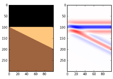
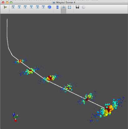
Still I was surprised when, chatting to Thomas Rapstine at the Geophysics Hackathon in Denver, he mentioned Joe Capriotti and Yaoguo Li, fellow researchers at Colorado School of Mines. Faced with the problem of building 3D earth models for simulating geophysical experiments — a problem we've faced with modelr.io — they hit on the idea of adapting Minecraft models. This is not just a gimmick, because Minecraft is specifically designed for simulating and manipulating landscapes.

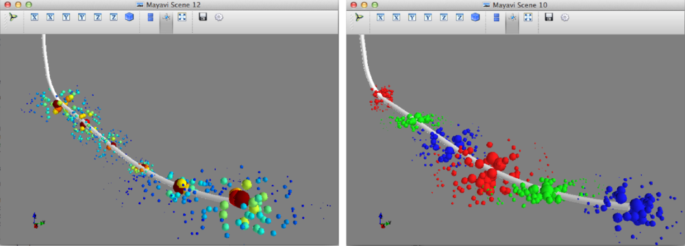
The Minecraft model (left) and synthetic gravity data (right). Image ©2014 SEG and Capriotti & Li. Used in acordance with SEG's permissions. 

If you'd like to dabble in geospatial Minecraft yourself, the FME software from Safe now has a standardized way to get Minecraft data into and out of the environment. Essentially they treat the blocks as point clouds (e.g. as you might get from Lidar or a laser scan), so they can do conventional operations, such as differences or filtering, with the software. They recorded a webinar on the subject yesterday.

Minecraft is here to stay

There are two other important angles to Minecraft, both good reasons why it will probably be around for a while, and probably both something to do with why Microsoft bought Mojang...

1. It is a programming gateway drug. Like web coding, and image processing, Minecraft might be another way to get people, especially young people, interested in computing. The tiny Linux machine Raspberry Pi comes with a version of the game with a full Python API, so you can control the game programmatically.  
2. Its potential beyond programming as a STEM teaching aid and engagement tool. Here's another example. Indeed, the United Nations is involved in Block By Block, an effort around collaborative public space design echoing the Blockholm project, an early attempt to explore social city planning in the tool.

All of which is enough to make me more curious about the crazy-sounding world my kids have built, with its Houston-like city planning: house, school, house, Home Sense, house, rocket launch pad...

References

Capriotti, J and Yaoguo Li (2014) Gravity and gravity gradient data: Understanding their information content through joint inversions. SEG Technical Program Expanded Abstracts 2014: pp. 1329-1333. DOI 10.1190/segam2014-1581.1 

The thumbnail image is from an image by Terry Madeley.

UPDATE: Thank you to Andy for pointing out that Yaoguo Li is a prof, not a student.

Six books about seismic analysis

Last year, I did a round-up of six books about seismic interpretation. A raft of new geophysics books recently, mostly from Cambridge, prompts this look at six volumes on seismic analysis — the more quantitative side of interpretation. We seem to be a bit hopeless at full-blown book reviews, and I certainly haven't read all of these books from cover to cover, but I thought I could at least mention them, and give you my first impressions.

If you have read any of these books, I'd love to hear what you think of them! Please leave a comment. 

Observation: none of these volumes mention compressive sensing, borehole seismic, microseismic, tight gas, or source rock plays. So I guess we can look forward to another batch in a year or two, when Cambridge realizes that people will probably buy anything with 3 or more of those words in the title. Even at $75 a go.

---

Quantitative Seismic Interpretation

Per Avseth, Tapan Mukerji and Gary Mavko (2005). Cambridge University Press, 408 pages, ISBN 978-0-521-15135-1. List price USD 91, $81.90 at Amazon.com, £45.79 at Amazon.co.uk

You have this book, right?

Every seismic interpreter that's thinking about rock properties, AVO, inversion, or anything beyond pure basin-scale geological interpretation needs this book. And the MATLAB scripts.

Rock Physics Handbook

Gary Mavko, Tapan Mukerji & Jack Dvorkin (2009). Cambridge University Press, 511 pages, ISBN 978-0-521-19910-0. List price USD 100, $92.41 at Amazon.com, £40.50 at Amazon.co.uk

If QSI is the book for quantitative interpreters, this is the book for people helping those interpreters. It's the Aki & Richards of rock physics. So if you like sums, and QSI left you feeling unsatisifed, buy this too. It also has lots of MATLAB scripts.

Seismic Reflections of Rock Properties

Jack Dvorkin, Mario Gutierrez & Dario Grana (2014). Cambridge University Press, 365 pages, ISBN 978-0-521-89919-2. List price USD 75, $67.50 at Amazon.com, £40.50 at Amazon.co.uk

This book seems to be a companion to The Rock Physics Handbook. It feels quite academic, though it doesn't contain too much maths. Instead, it's more like a systematic catalog of log models — exploring the full range of seismic responses to rock properies.

Practical Seismic Data Analysis

Hua-Wei Zhou (2014). Cambridge University Press, 496 pages, ISBN 978-0-521-19910-0. List price USD 75, $67.50 at Amazon.com, £40.50 at Amazon.co.uk

Zhou is a professor at the University of Houston. His book leans towards imaging and velocity analysis — it's not really about interpretation. If you're into signal processing and tomography, this is the book for you. Mostly black and white, the book has lots of exercises (no solutions though).

Seismic Amplitude: An Interpreter's Handbook

Rob Simm & Mike Bacon (2014). Cambridge University Press, 279 pages, ISBN 978-1-107-01150-2 (hardback). List price USD 80, $72 at Amazon.com, £40.50 at Amazon.co.uk

Simm is a legend in quantitative interpretation and the similarly lauded Bacon is at Ikon, the pre-eminent rock physics company. These guys know their stuff, and they've filled this superbly illustrated book with the essentials. It belongs on every interpreter's desk.

Seismic Data Analysis Techniques...

Enwenode Onajite (2013). Elsevier. 256 pages, ISBN 978-0124200234. List price USD 130, $113.40 at Amazon.com. £74.91 at Amazon.co.uk.

This is the only book of the collection I don't have. From the preview I'd say it's aimed at undergraduates. It starts with a petroleum geology primer, then covers seismic acquisition, and seems to focus on processing, with a little on interpretation. The figures look rather weak, compared to the other books here. Not recommended, not at this price.

NOTE These prices are Amazon's discounted prices and are subject to change. The links contain a tag that gets us commission, but does not change the price to you. You can almost certainly buy these books elsewhere. 

How much rock was erupted from Mt St Helens?

One of the reasons we struggle when learning a new skill is not necessarily because this thing is inherently hard, or that we are dim. We just don't yet have enough context for all the connecting ideas to, well, connect. With this in mind I wrote this introductory demo for my Creative Geocomputing class, and tried it out in the garage attached to START Houston, when we ran the course there a few weeks ago.

I walked through the process of transforming USGS text files to data graphics. The motivation was to try to answer the question: How much rock was erupted from Mount St Helens?

This gorgeous data set can be reworked to serve a lot of programming and data manipulation practice, and just have fun solving problems. My goal was to maintain a coherent stream of instructions, especially for folks who have never written a line of code before. The challenge, I found, is anticipating when words, phrases, and syntax are being heard like a foriegn language (as indeed they are), and to cope by augmenting with spoken narrative.

Text file to 3D plot

To start, we'll import a code library called NumPy that's great for crunching numbers, and we'll abbreviate it with the nickname np:

>>> import numpy as np

Then we can use one of its functions to load the text file into an array we'll call data:

>>> data = np.loadtxt('z_after.txt')

The variable data is a 2-dimensional array (matrix) of numbers. It has an attribute that we can call upon, called shape, that holds the number of elements it has in each dimension,

>>> data.shape
(1370, 949)

If we want to make a plot of this data, we might want to take a look at the range of the elements in the array, we can call the peak-to-peak method on data,

>>> data.ptp()
41134.0

Whoa, something's not right, there's not a surface on earth that has a min to max elevation that large. Let's dig a little deeper. The highest point on the surface is,

>>> np.amax(data)
8367.0

Which looks to the adequately trained eye like a reasonable elevation value with units of feet. Let's look at the minimum value of the array,

>>> np.amin(data)
-32767.0 

OK, here's the problem. GIS people might recognize this as a null value for elevation data, but since we aren't assuming any knowledge of GIS formats and data standards, we can simply replace the values in the array with not-a-number (NaN), so they won't contaminate our plot.

>>> data[data==-32767.0] = np.nan

To view this surface in 3D we can import the mlab module from Mayavi, 

>>> from mayavi import mlab

Finally we call the surface function from mlab, and pass the input data, and a colormap keyword to activate a geographically inspired colormap, and a vertical scale coefficient.

>>> mlab.surf(data,
              colormap='gist_earth',
              warp_scale=0.05)

After applying the same procedure to the pre-eruption digits, we're ready to do some calculations and visualize the result to reveal the output and its fascinating characteristics. Read more in the IPython Notebook.

If this 10 minute introduction is compelling and you'd like to learn how to wrangle data like this, sign up for the two-day version of this course next week in Calgary. 

Relentlessly practical

This is one of my favourite knowledge sharing stories.

A farmer in my community had a problem with one of his cows — it was seriously unwell. He asked one of the old local farmers about the symptoms, and was told, “Oh yes, one of my herd had the same thing last summer. I gave her a cup of brandy and four aspirins every night for a week.” The young farmer went off and did this, but the poor cow got steadily worse and died. When he saw the old farmer next he told him, more than a little accusingly, “I did what you said, and the cow died anyway.” The old geezer looked into the distance and just said, “Yep, so did mine.”

Incomplete information can be less useful than no information. Yet incomplete information has somehow become our specialty in applied geoscience. How often do we share methods, results, or case studies without the critical details that would make it useful information? That is, not just marketing, or resumé padding. Inded, I heard this week that one large US operator will not approve a publication that does include these critical details! And we call ourselves scientists...

Completeness mandatory

Thankfully, Last month The Leading Edge — the magazine of the SEG — started a new tutorial column, edited by me. Well, I say 'edited', I'm just the person that pesters prospective authors until they give in and send me a manuscript. Tad Smith, Don Herron, and Jenny Kucera are the people that make it actually happen. But I get to take all the credit.

When I was asked about it, I suggested two things:

1. Make each tutorial reproducible by publishing the code that makes the figures.
2. Make the words, the data, and the code completely open and shareable. 

To my delight and, I admit, slight surprise, they said 'Sure!'. So the words are published under an open license (Creative Commons Attribution-ShareAlike, the same license for re-use that most of Wikipedia has), the tutorials use open data for everything, and the code is openly available and free to re-use. Complete transparency.

There's another interesting aspect to how the column is turning out. The first two episodes tell part of the story in IPython Notebook, a truly amazing executable writing environment that we've written about before. This enables you to seamlessly stich together text, code, and plots (left). If you know a bit of Python, or want to start learning it right now this second, go give wakari.io a try. It's pretty great. (If you really like it, come and learn more with us!).

Read the first tutorial: Hall, M. (2014). Smoothing surfaces and attributes. The Leading Edge, 33(2), 128–129. doi: 10.1190/tle33020128.1. A version of it is also on SEG Wiki, and you can read the IPython Notebook at nbviewer.org.

Do you fancy authoring something for this column? Wonderful — please do! Here are the author instructions. If you have an idea for something, please drop me a line, let's talk about how to make it relentlessly practical.

Creating in the classroom

The day before the Atlantic Geoscience Colloquium, I hosted a one-day workshop on geoscience computing to 26 maritime geoscientists. This was my third time running this course. Each time it has needed tailoring and new exercises to suit the crowd; a room full of signal-processing seismologists has a different set of familiarities than one packed with hydrologists, petrologists, and cartographers. 

Easier to consume than create

At the start of the day, I asked people to write down the top five things they spend time doing with computers. I wanted a record of the tools people use, but also to take collective stock of our creative, as opposed to consumptive, work patterns. Here's the result (right).

My assertion was that even technical people spend most of their time in relatively passive acts of consumption — browsing, emailing, and so on. Creative acts like writing, drawing, or using software were in the minority, and only a small sliver of time is spent programming. Instead of filing into a darkened room and listening to PowerPoint slides, or copying lectures notes from a chalkboard, this course was going to be different. Participation mandatory.

My goal is not to turn every geoscientist into a software developer, but to better our capacity to communicate with computers. Giving people resources and training to master this medium that warrants a new kind of creative expression. Through coaching, tutorials, and exercises, we can support and encourage each other in more powerful ways of thinking. Moreover, we can accelerate learning, and demystify computer programming by deliberately designing exercises that are familiar and relevant to geoscientists. 

Scientific computing

In the first few hours students learned about syntax, built-in functions, how and why to define and call functions, as well as how to tap into external code libraries and documentation. Scientific computing is not necessarily about algorithm theory, passing unit tests, or designing better user experiences. Scientists are above all interested in data, and data processes, helped along by rich graphical displays for story telling.

Elevation model (left), and slope magnitude (right), Cape Breton, Nova Scotia. Click to enlarge.

In the final exercise of the afternoon, students produced a topography map of Nova Scotia (above left) from a georeferenced tiff. Sure, it's the kind of thing that can be done with a GIS, and that is precisely the point. We also computed some statistical properties to answer questions like, "what is the average elevation of the province?", or "what is the steepest part of the province?". Students learned about doing calculus on surfaces as well as plotting their results. 

Programming is a learnable skill through deliberate practice. What's more, if there is one thing you can teach yourself on the internet, it is computer programming. Perhaps what is scarce though, is finding the time to commit to a training regimen. It's rare that any busy student or working professional can set aside a chunk of 8 hours to engage in some deliberate coaching and practice. A huge bonus is to do it alongside a cohort of like-minded individuals willing and motivated to endure the same graft. This is why we're so excited to offer this experience — the time, help, and support to get on with it.

How can I take the course?

We've scheduled two more episodes for the spring, conveniently aligned with the 2014 AAPG convention in Houston, and the 2014 CSPG / CSEG convention in Calgary. It would be great to see you there!

  

Or maybe a customized in-house course would suit your needs better? We'd love to help. Get in touch.

To make up microseismic

I am not a proponent of making up fictitious data, but for the purposes of demonstrating technology, why not? This post is the third in a three-part follow-up from the private beta I did in Calgary a few weeks ago. You can check out the IPython Notebook version too. If you want more of this in person, sign up at the bottom or drop us a line. We want these examples to be easily readable, especially if you aren't a coder, so please let us know how we are doing.

Start by importing some packages that you'll need into the workspace,

%pylab inline

import numpy as np
from scipy.interpolate import splprep, splev
import matplotlib.pyplot as plt
import mayavi.mlab as mplt
from mpl_toolkits.mplot3d import Axes3D

Define a borehole path

We define the trajectory of a borehole, using a series of x, y, z points, and make each component of the borehole an array. If we had a real well, we load the numbers from the deviation survey just the same.

trajectory = np.array([[   0,   0,    0],
                       [   0,   0, -100],
                       [   0,   0, -200],
                       [   5,   0, -300],
                       [  10,  10, -400],
                       [  20,  20, -500],
                       [  40,  80, -650],
                       [ 160, 160, -700],
                       [ 600, 400, -800],
                       [1500, 960, -800]])
x = trajectory[:,0]
y = trajectory[:,1]
z = trajectory[:,2]

But since we want the borehole to be continuous and smoothly shaped, we can up-sample the borehole by finding the B-spline representation of the well path,

smoothness = 3.0
spline_order = 3
nest = -1 # estimate of number of knots needed (-1 = maximal)
knot_points, u = splprep([x,y,z], s=smoothness, k=spline_order, nest=-1)

# Evaluate spline, including interpolated points
x_int, y_int, z_int = splev(np.linspace(0, 1, 400), knot_points)

plt.gca(projection='3d')
plt.plot(x_int, y_int, z_int, color='grey', lw=3, alpha=0.75)
plt.show()

Define frac ports

Let's define a completion program so that our wellbore has 6 frac stages,

number_of_fracs = 6

and let's make it so that each one emanates from equally spaced frac ports spanning the bottom two-thirds of the well.

x_frac, y_frac, z_frac = splev(np.linspace(0.33, 1, number_of_fracs), knot_points)

Make a set of 3D axes, so we can plot the well path and the frac ports.

ax = plt.axes(projection='3d')
ax.plot(x_int, y_int, z_int, color='grey',
        lw=3, alpha=0.75)
ax.scatter(x_frac, y_frac, z_frac,
        s=100, c='grey')
plt.show()

Set a colour for each stage by cycling through red, green, and blue,

stage_color = []
for i in np.arange(number_of_fracs):
    color = (1.0, 0.1, 0.1)
    stage_color.append(np.roll(color, i))
stage_color = tuple(map(tuple, stage_color))

Define microseismic points

One approach is to create some dimensions for each frac stage and generate 100 points randomly within each zone. Each frac has an x half-length, y half-length, and z half-length. Let's also vary these randomly for each of the 6 stages. Define the dimensions for each stage:

frac_dims = []
half_extents = [500, 1000, 250]
for i in range(number_of_fracs):
    for j in range(len(half_extents)):
        dim = np.random.rand(3)[j] * half_extents[j]
        frac_dims.append(dim)  
frac_dims = np.reshape(frac_dims, (number_of_fracs, 3))

Plot microseismic point clouds with 100 points for each stage. The following code should launch a 3D viewer scene in its own window:

size_scalar = 100000
mplt.plot3d(x_int, y_int, z_int, tube_radius=10)
for i in range(number_of_fracs):
    x_cloud = frac_dims[i,0] * (np.random.rand(100) - 0.5)
    y_cloud = frac_dims[i,1] * (np.random.rand(100) - 0.5)
    z_cloud = frac_dims[i,2] * (np.random.rand(100) - 0.5)

    x_event = x_frac[i] + x_cloud
    y_event = y_frac[i] + y_cloud     
    z_event = z_frac[i] + z_cloud
    
    # Let's make the size of each point inversely proportional 
    # to the distance from the frac port
    size = size_scalar / ((x_cloud**2 + y_cloud**2 + z_cloud**2)**0.002)
    
    mplt.points3d(x_event, y_event, z_event, size, mode='sphere', colormap='jet')

You can swap out the last line in the code block above with mplt.points3d(x_event, y_event, z_event, size, mode='sphere', color=stage_color[i]) to colour each event by its corresponding stage.

A day of geocomputing

I will be in Calgary in the new year and running a one-day version of this new course. To start building your own tools, pick a date and sign up:

    

To make a wedge

We'll need a wavelet like the one we made last time. We could import it, if we've made one, but SciPy also has one so we can save ourselves the trouble. Remember to put %pylab inline at the top if using IPython notebook.

import numpy as np
from scipy.signal import ricker
import matplotlib.pyplot as plt

Now we need to make a physical earth model with three rock layers. In this example, let's make an acoustic impedance earth model. To keep it simple, let's define the earth model with two-way-travel time along the vertical axis (as opposed to depth). There are number of ways you could describe a wedge using math, and you could probably come up with a way that is better than mine. Here's a way:

nsamps, ntraces = [600, 500]
rock_names = ['shale 1', 'sand', 'shale 2']
rock_grid = np.zeros((n_samples, n_traces))

def make_wedge(n_samples, n_traces, layer_1_thickness, start_wedge, end_wedge):
    for j in np.arange(n_traces): 
        for i in np.arange(n_samples):      
            if i <= layer_1_thickness:      
                rock_grid[i][j] = 1    
            if i > layer_1_thickness:         
                rock_grid[i][j] = 3    
                if j >= start_wedge and i - layer_1_thickness < j-start_wedge: 
                    rock_grid[i][j] = 2
                    if j >= end_wedge and i > layer_1_thickness+(end_wedge-start_wedge):
                        rock_grid[i][j] = 3
    return rock_grid

Let's insert some numbers into our wedge function and make a particular geometry.

layer_1_thickness = 200
start_wedge = 50
end_wedge = 250
rock_grid = make_wedge(n_samples, n_traces, 
            layer_1_thickness, start_wedge, 
            end_wedge)

plt.imshow(rock_grid, cmap='copper_r')

Now we can give each layer in the wedge properties.

vp = np.array([3300., 3200., 3300.]) 
rho = np.array([2600., 2550., 2650.]) 
AI = vp*rho
AI = AI / 10e6 # re-scale (optional step)

Then assign values assign them accordingly to every sample in the rock model.

model = np.copy(rock_grid)
model[rock_grid == 1] = AI[0]
model[rock_grid == 2] = AI[1]
model[rock_grid == 3] = AI[2]

plt.imshow(model, cmap='Spectral')
plt.colorbar()
plt.title('Impedances')

Now we can compute the reflection coefficients. I have left out a plot of the reflection coefficients, but you can check it out in the full version in the nbviewer

upper = model[:-1][:]
lower = model[1:][:]
rc = (lower - upper) / (lower + upper)
maxrc = abs(np.amax(rc))

Now we make the wavelet interact with the model using convolution. The convolution function already exists in the SciPy signal library, so we can just import it.

from scipy.signal import convolve
def make_synth(f):
    synth = np.zeros((n_samples+len(t)-2, n_traces))
    wavelet = ricker(512, 1e3/(4.*f))
    wavelet = wavelet / max(wavelet)   # normalize
    for k in range(n_traces):
        synth[:,k] = convolve(rc[:,k], wavelet)
    synth = synth[ np.ceil(len(wavelet))/2 : -np.ceil(len(wavelet))/2, : ]
    return synth

Finally, we plot the results.

frequencies = array([5, 10, 15])
plt.figure(figsize = (15, 4))
for i in np.arange(len(frequencies)):
    this_plot = make_synth(frequencies[i])
    plt.subplot(1, len(frequencies), i+1)
    plt.imshow(this_plot, cmap='RdBu', vmax=maxrc, vmin=-maxrc, aspect=1)
    plt.title( '%d Hz wavelet' % freqs[i] )
    plt.grid()
    plt.axis('tight')
    
    # Add some labels
    for i, names in enumerate(rock_names):
        plt.text(400, 100+((end_wedge-start_wedge)*i+1), names,
                 fontsize=14, color='gray',
                 horizontalalignment='center',
                 verticalalignment='center')

 

That's it. As you can see, the marriage of building mathematical functions and plotting them can be a really powerful tool you can apply to almost any physical problem you happen to find yourself working on.

You can access the full version in the nbviewer. It has a few more figures than what is shown in this post.

A day of geocomputing

I will be in Calgary in the new year and running a one-day version of this new course. To start building your own tools, pick a date and sign up:

    

To plot a wavelet

As I mentioned last time, a good starting point for geophysical computing is to write a mathematical function describing a seismic pulse. The IPython Notebook is designed to be used seamlessly with Matplotlib, which is nice because we can throw our function on graph and see if we were right. When you start your own notebook, type

ipython notebook --pylab inline

We'll make use of a few functions within NumPy, a workhorse to do the computational heavy-lifting, and Matplotlib, a plotting library.

import numpy as np
import matplotlib.pyplot as plt

Next, we can write some code that defines a function called ricker. It computes a Ricker wavelet for a range of discrete time-values t and dominant frequencies, f:

def ricker(f, length=0.512, dt=0.001):
    t = np.linspace(-length/2, (length-dt)/2, length/dt)
    y = (1.-2.*(np.pi**2)*(f**2)*(t**2))*np.exp(-(np.pi**2)*(f**2)*(t**2))
    return t, y

Here the function needs 3 input parameters; frequency, f, the length of time over which we want it to be defined, and the sample rate of the signal, dt. Calling the function returns two arrays, the time axis t, and the value of the function, y.

To create a 5 Hz Ricker wavelet, assign the value of 5 to the variable f, and pass it into the function like so,

f = 5
t, y = ricker (f)

To plot the result,

plt.plot(t, y)

But with a few more commands, we can improve the cosmetics,

plt.figure(figsize=(7,4))
plt.plot( t, y, lw=2, color='black', alpha=0.5)
plt.fill_between(t, y, 0,  y > 0.0, interpolate=False, hold=True, color='blue', alpha = 0.5)
plt.fill_between(t, y, 0, y < 0.0, interpolate=False, hold=True, color='red', alpha = 0.5)

# Axes configuration and settings (optional)
plt.title('%d Hz Ricker wavelet' %f, fontsize = 16 )
plt.xlabel( 'two-way time (s)', fontsize = 14)
plt.ylabel('amplitude', fontsize = 14)
plt.ylim((-1.1,1.1))
plt.xlim((min(t),max(t)))
plt.grid()
plt.show()

Next up, we'll make this wavelet interact with a model of the earth using some math. Let me know if you get this up and running on your own.

Let's do it

It's short notice, but I'll be in Calgary again early in the new year, and I will be running a one-day version of this new course. To start building your own tools, pick a date and sign up:

    

Coding to tell stories

Last week, I was in Calgary on family business, but I took an afternoon to host a 'private beta' for a short course that I am creating for geoscience computing. I invited about twelve familiar faces who would be provide gentle and constuctive feedback. In the end, thirteen geophysicists turned up, seven of whom I hadn't met before. So much for familiarity.

I spent about two and half hours stepping through the basics of the Python programming language, which I consider essential material — getting set up with Python via Enthought Canopy, basic syntax, and so on. In the last hour of the afternoon, I steamed through a number of geoscientific examples to showcase exercises for this would-be course. 

Here are three that went over well. Next week, I'll reveal the code for making these images. I might even have a go at converting some of my teaching materials from IPython Notebook to HTML:

To plot a wavelet

The Ricker wavelet is a simple analytic function that is used throughout seismology. This curvaceous waveform is easily described by a single variable, the dominant frequency of its many contituents frequencies. Every geophysicist and their cat should know how to plot one: 

To make a wedge

Once you can build a wavelet, the next step is to make that wavelet interact with the earth. The convolution of the wavelet with this 3-layer impedance model yields a synthetic seismogram suitable for calibrating seismic signals to subtle stratigraphic geometries. Every interpreter should know how to build a wedge, with site-specific estimates of wavelet shape and impedance contrasts. Wedge models are important in all instances of dipping and truncated layers at or below the limit of seismic resolution. So basically they are useful all of the time. 

To make a 3D viewer

The capacity of Python to create stunning graphical displays with merely a few (thoughtful) lines of code seemed to resonate with people. But make no mistake, it is not easy to wade through the hundreds of function arguments to access this power and richness. It takes practice. It appears to me that practicing and training to search for and then read documentation, is the bridge that carries people from the mundane to the empowered.

This dry-run suggested to me that there are at least two markets for training here. One is a place for showing what's possible — "Here's what we can do, now let’s go and build it". The other, more arduous path is the coaching, support, and resources to motivate students through the hard graft that follows. The former is centered on problem solving, the latter is on problem finding, where the work and creativity and sweat is. 

Would you take this course? What would you want to learn? What problem would you bring to solve?

Update on 2013-12-10 13:17 by Evan Bianco

Update: the first follow-up post in this series is a code-based tutorial on how to plot a wavelet, and has an announcement about two 1-day events I will be holding in Calgary in the new year (January 10, and January 13, 2014).

Plant a seed for science and tech

Cruising around the web last weekend looking for geosciencey Christmas presents, coupled with having 3 kids (aged 9, 5, and 3) to entertain and educate, I just realized I have a long list of awesome toys to share. Well, I say toys, but these amazing things are almost in a class of their own...

Bigshot camera

A full kit for a child to build his or her own camera, and it's only $89. Probably best suited to those aged 7 up to about 12. Features:

• comes with everything you need, including a screwdriver,
• a crank instead of a battery,
• multiple lenses including anaglyphic 3D,
• a set of online tutorials about the components and how they work — enlightening!

LittleBits

Epic. For kids (and others) that aren't quite ready for a soldering iron, these magentic blocks just work. There are blocks for power, for input (like this pressure sensor), and for output. They can, and should, be combined with each other and anything else (Lego, Meccano, straws, dinosaurs) for maximum effect. Wonderful.

Anything at all from SparkFun

... and there's Adafruit too. I know we had Tandy or RadioShack or whatever in the early 1980s, but we didn't have the Internet. So life was, you know, hard. No longer. Everything at SparkFun is affordable, well-designed, well-documented, and—well—fun. I mean, who wouldn't want to build their own Simon Says? 

And this is just a fraction of what's out there... Lego MINDSTORMS for the bigger kids, GoldieBlox for smaller kids, Raspberry Pi for the teens. I get very excited when I think about what this means for the future of invention, creativity, and applied science. 

Even more exciting, it's us grown-ups that get to help them explore all this fun. Where will you start?