To make up microseismic

I am not a proponent of making up fictitious data, but for the purposes of demonstrating technology, why not? This post is the third in a three-part follow-up from the private beta I did in Calgary a few weeks ago. You can check out the IPython Notebook version too. If you want more of this in person, sign up at the bottom or drop us a line. We want these examples to be easily readable, especially if you aren't a coder, so please let us know how we are doing.

Start by importing some packages that you'll need into the workspace,

%pylab inline

import numpy as np
from scipy.interpolate import splprep, splev
import matplotlib.pyplot as plt
import mayavi.mlab as mplt
from mpl_toolkits.mplot3d import Axes3D

Define a borehole path

We define the trajectory of a borehole, using a series of x, y, z points, and make each component of the borehole an array. If we had a real well, we load the numbers from the deviation survey just the same.

trajectory = np.array([[   0,   0,    0],
                       [   0,   0, -100],
                       [   0,   0, -200],
                       [   5,   0, -300],
                       [  10,  10, -400],
                       [  20,  20, -500],
                       [  40,  80, -650],
                       [ 160, 160, -700],
                       [ 600, 400, -800],
                       [1500, 960, -800]])
x = trajectory[:,0]
y = trajectory[:,1]
z = trajectory[:,2]

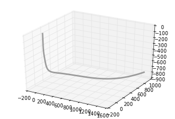
But since we want the borehole to be continuous and smoothly shaped, we can up-sample the borehole by finding the B-spline representation of the well path,

smoothness = 3.0
spline_order = 3
nest = -1 # estimate of number of knots needed (-1 = maximal)
knot_points, u = splprep([x,y,z], s=smoothness, k=spline_order, nest=-1)

# Evaluate spline, including interpolated points
x_int, y_int, z_int = splev(np.linspace(0, 1, 400), knot_points)

plt.gca(projection='3d')
plt.plot(x_int, y_int, z_int, color='grey', lw=3, alpha=0.75)
plt.show()

Define frac ports

Let's define a completion program so that our wellbore has 6 frac stages,

number_of_fracs = 6

and let's make it so that each one emanates from equally spaced frac ports spanning the bottom two-thirds of the well.

x_frac, y_frac, z_frac = splev(np.linspace(0.33, 1, number_of_fracs), knot_points)

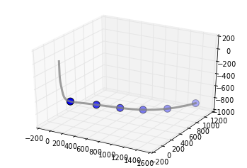Make a set of 3D axes, so we can plot the well path and the frac ports.

ax = plt.axes(projection='3d')
ax.plot(x_int, y_int, z_int, color='grey',
        lw=3, alpha=0.75)
ax.scatter(x_frac, y_frac, z_frac,
        s=100, c='grey')
plt.show()

Set a colour for each stage by cycling through red, green, and blue,

stage_color = []
for i in np.arange(number_of_fracs):
    color = (1.0, 0.1, 0.1)
    stage_color.append(np.roll(color, i))
stage_color = tuple(map(tuple, stage_color))

Define microseismic points

One approach is to create some dimensions for each frac stage and generate 100 points randomly within each zone. Each frac has an x half-length, y half-length, and z half-length. Let's also vary these randomly for each of the 6 stages. Define the dimensions for each stage:

frac_dims = []
half_extents = [500, 1000, 250]
for i in range(number_of_fracs):
    for j in range(len(half_extents)):
        dim = np.random.rand(3)[j] * half_extents[j]
        frac_dims.append(dim)  
frac_dims = np.reshape(frac_dims, (number_of_fracs, 3))

Plot microseismic point clouds with 100 points for each stage. The following code should launch a 3D viewer scene in its own window:

size_scalar = 100000
mplt.plot3d(x_int, y_int, z_int, tube_radius=10)
for i in range(number_of_fracs):
    x_cloud = frac_dims[i,0] * (np.random.rand(100) - 0.5)
    y_cloud = frac_dims[i,1] * (np.random.rand(100) - 0.5)
    z_cloud = frac_dims[i,2] * (np.random.rand(100) - 0.5)

    x_event = x_frac[i] + x_cloud
    y_event = y_frac[i] + y_cloud     
    z_event = z_frac[i] + z_cloud
    
    # Let's make the size of each point inversely proportional 
    # to the distance from the frac port
    size = size_scalar / ((x_cloud**2 + y_cloud**2 + z_cloud**2)**0.002)
    
    mplt.points3d(x_event, y_event, z_event, size, mode='sphere', colormap='jet')

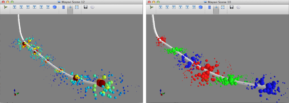
You can swap out the last line in the code block above with mplt.points3d(x_event, y_event, z_event, size, mode='sphere', color=stage_color[i]) to colour each event by its corresponding stage.

A day of geocomputing

I will be in Calgary in the new year and running a one-day version of this new course. To start building your own tools, pick a date and sign up:

    

The future is uncertain

Image: Repsol, SEG. Click for the abstract.

SEG Day 2. In the session entitled Exploration and Uncertainty Analysis, I was underwhelmed with the few talks that I attended, except for the last one of the session entitled, Measuring time-map uncertainty. 

Static uncertainty

It is commonly uttered that different data processing companies will produce different results; seismic processing is non-unique, and so on. But rarely do I get to see real examples of the kind of variances that can occur. Bruce Blake from Repsol showed seismic imaging results that came back from a number of contractors. The results were truly shocking. The example he showed was an extreme case of uncertainty caused by inadequate static solutions caused by the large sand dunes in Libya. The key point for me is exemplified by the figure shown on the right: the image from one vendor suggests a syncline, the image from the other suggest an anticline. Beware!

A hole in the theory

In the borehole sonic session, Xinding Fang, a student from MIT, reinforced a subtle but profound idea: it is tricky to measure the speed of sound in a rock when you drill a hole into it. The hole changes the stress field, and induces an anisotropic stiffness around the circumference of the borehole where sonic tools make their measurements. And since waves take the shortest travel path from source to receiver, speeds that are measured in the presence of an artificial stress are wrong.

Image: Xindang Fang, SEG. Click for the abstract.

The bigger issue here that Xinding has elucidated is that we routinely use sonic logs to make time-depth relationships and tie wells, especially in the absence of a check-shot survey. If it works, it works, but if ever discrepancies exists between seismic and well, the interpreter applies a stretch or a squeeze without much thought. Some may blame the discrepancy on dispersion alone, but that's evidently too narrow. Indeed, we rarely bother to investigate the reasons.

There's a profound point here. We have to drop the assumption that logs are the 'geological' truth upon which to hang an interpretation. We have to realize that the act of making the measurement changes the very thing we want to measure.