x lines of Python: read and write a shapefile

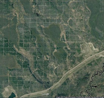
Shapefiles are a sort-of-open format for geospatial vector data. They can encode points, lines, and polygons, plus attributes of those objects, optionally bundled into groups. I say 'sort-of-open' because the format is well-known and widely used, but it is maintained and policed, so to speak, by ESRI, the company behind ArcGIS. It's a slightly weird (annoying) format because 'a shapefile' is actually a collection of files, only one of which is the eponymous SHP file. 

Today we're going to read a SHP file, change its Coordinate Reference System (CRS), add a new attribute, and save a new file in two different formats. All in x lines of Python, where x is a small number. To do all this, we need to add a new toolbox to our xlines virtual environment: geopandas, which is a geospatial flavour of the popular data management tool pandas.

Here's the full rundown of the workflow, where each item is a line of Python:

  1. Open the shapefile with fiona (i.e. not using geopandas yet).
  2. Inspect its contents.
  3. Open the shapefile again, this time with geopandas.
  4. Inspect the resulting GeoDataFrame in various ways.
  5. Check the CRS of the data.
  6. Change the CRS of the GeoDataFrame.
  7. Compute a new attribute.
  8. Write the new shapefile.
  9. Write the GeoDataFrame as a GeoJSON file too.

By the way, if you have not come across EPSG codes yet for CRS descriptions, they are the only way to go. This dataset is initially in EPSG 4267 (NAD27 geographic coordinates) but we change it to EPSG 26920 (NAD83 UTM20N projection).

Several bits of our workflow are optional. The core part of the code, items 3, 6, 7, and 8, are just a few lines of Python:

    import geopandas as gpd
    gdf = gpd.read_file('data_in.shp')
    gdf = gdf.to_crs({'init': 'epsg:26920'})
    gdf['seafl_twt'] = 2 * 1000 * gdf.Water_Dept / 1485
    gdf.to_file('data_out.shp')

That's it! 

As in all these posts, you can follow along with the code in the Jupyter Notebook.

Laying out a seismic survey

Cutlines for a dense 3D survey at Surmont field, Alberta, Canada. Image: Google Maps.

Cutlines for a dense 3D survey at Surmont field, Alberta, Canada. Image: Google Maps.

Cutlines for a dense 3D survey at Surmont field, Alberta, Canada. Image: Google Maps.There are a number of ways to lay out sources and receivers for a 3D seismic survey. In forested areas, a designer may choose a pattern that minimizes the number of trees that need to be felled. Where land access is easier, designers may opt for a pattern that is efficient for the recording crew to deploy and pick up receivers. However, no matter what survey pattern used, most geometries consist of receivers strung together along receiver lines and source points placed along source lines. The pairing of source points with live receiver stations comprises the collection of traces that go into making a seismic volume.

An orthogonal surface pattern, with receiver lines laid out perpendicular to the source lines, is the simplest surface geometry to think about. This pattern can be specified over an area of interest by merely choosing the spacing interval between lines well as the station intervals along the lines. For instance:

xmi = 575000        # Easting of bottom-left corner of grid (m)
ymi = 4710000       # Northing of bottom-left corner (m)
SL = 600            # Source line interval (m)
RL = 600            # Receiver line interval (m)
si = 100            # Source point interval (m)
ri = 100            # Receiver point interval (m)
x = 3000            # x extent of survey (m)
y = 1800            # y extent of survey (m)

We can calculate the number of receiver lines and source lines, as well as the number of receivers and sources for each.

# Calculate the number of receiver and source lines.
rlines = int(y/RL) + 1
slines = int(x/SL) + 1

# Calculate the number of points per line (add 2 to straddle the edges). 
rperline = int(x/ri) + 2 
sperline = int(y/si) + 2

# Offset the receiver points.
shiftx = -si/2.
shifty = -ri/2.

Computing coordinates

We create a list of x and y coordinates with a nested list comprehension — essentially a compact way to write 'for' loops in Python — that iterates over all the stations along the line, and all the lines in the survey.

# Find x and y coordinates of receivers and sources.
rcvrx = [xmi+rcvr*ri+shifty for line in range(rlines) for rcvr in range(rperline)]
rcvry = [ymi+line*RL+shiftx for line in range(rlines) for rcvr in range(rperline)]

srcx = [xmi+line*SL for line in range(slines) for src in range(sperline)]
srcy = [ymi+src*si for line in range(slines) for src in range(sperline)]

To make a map of the ideal surface locations, we simply pass this list of x and y coordinates to a scatter plot:

srcs_recs_pattern.png

Plotting these lists is useful, but it is rather limited by itself. We're probably going to want to do more calculations with these points — midpoints, azimuth distributions, and so on — and put these data on a real map. What we need is to insert these coordinates into a more flexible data structure that can hold additional information.

Shapely, Pandas, and GeoPandas

Shapely is a library for creating and manipulating geometric objects like points, lines, and polygons. For example, Shapely can easily calculate the (x, y) coordinates halfway along a straight line between two points.

Pandas provides high-performance, easy-to-use data structures and data analysis tools, designed to make working with tabular data easy. The two primary data structures of Pandas are:

  • Series — a one-dimensional labelled array capable of holding any data type (strings, integers, floating point numbers, lists, objects, etc.)
  • DataFrame — a 2-dimensional labelled data structure where the columns can contain many different types of data. This is similar to the NumPy structured array but much easier to use.

GeoPandas combines the capabilities of Shapely and Pandas and greatly simplifies geospatial operations in Python, without the need for a spatial database. GeoDataFrames are a special case of DataFrames that are specifically for representing geospatial data via a geometry column. One awesome thing about GeoDataFrame objects is they have methods for saving data to shapefiles.

So let's make a set of (x,y) pairs for receivers and sources, then make Point objects using Shapely, and in turn add those to GeoDataFrame objects, which we can write out as shapefiles:

# Zip into x,y pairs.
rcvrxy = zip(rcvrx, rcvry)
srcxy = zip(srcx, srcy)

# Create lists of shapely Point objects.
rcvrs = [Point(x,y) for x,y in rcvrxy]
srcs = [Point(x,y) for x,y in srcxy]

# Add lists to GeoPandas GeoDataFrame objects.
receivers = GeoDataFrame({'geometry': rcvrs})
sources = GeoDataFrame({'geometry': srcs})

# Save the GeoDataFrames as shapefiles.
receivers.to_file('receivers.shp')
sources.to_file('sources.shp')

It's a cinch to fire up QGIS and load these files as layers on top of a satellite image or physical topography map. As a survey designer, we can now add, delete, and move source and receiver points based on topography and land issues, sending the data back to Python for further analysis.

seismic_GIS_physical.png

All the code used in this post is in an IPython notebook. You can read it, and even execute it yourself. Put your own data in there and see how it comes out!

NEWSFLASH — If you think the geoscientists in your company would like to learn how to play with geological and geophysical models and data — exploring seismic acquisition, or novel well log displays — we can come and get you started! Best of all, we'll help you get up and running on your own data and your own ideas.

If you or your company needs a dose of creative geocomputing, check out our new geocomputing course brochure, and give us a shout if you have any questions. We're now booking for 2015.

Creating in the classroom

The day before the Atlantic Geoscience Colloquium, I hosted a one-day workshop on geoscience computing to 26 maritime geoscientists. This was my third time running this course. Each time it has needed tailoring and new exercises to suit the crowd; a room full of signal-processing seismologists has a different set of familiarities than one packed with hydrologists, petrologists, and cartographers. 

Easier to consume than create

At the start of the day, I asked people to write down the top five things they spend time doing with computers. I wanted a record of the tools people use, but also to take collective stock of our creative, as opposed to consumptive, work patterns. Here's the result (right).

My assertion was that even technical people spend most of their time in relatively passive acts of consumption — browsing, emailing, and so on. Creative acts like writing, drawing, or using software were in the minority, and only a small sliver of time is spent programming. Instead of filing into a darkened room and listening to PowerPoint slides, or copying lectures notes from a chalkboard, this course was going to be different. Participation mandatory.

My goal is not to turn every geoscientist into a software developer, but to better our capacity to communicate with computers. Giving people resources and training to master this medium that warrants a new kind of creative expression. Through coaching, tutorials, and exercises, we can support and encourage each other in more powerful ways of thinking. Moreover, we can accelerate learning, and demystify computer programming by deliberately designing exercises that are familiar and relevant to geoscientists. 

Scientific computing

In the first few hours students learned about syntax, built-in functions, how and why to define and call functions, as well as how to tap into external code libraries and documentation. Scientific computing is not necessarily about algorithm theory, passing unit tests, or designing better user experiences. Scientists are above all interested in data, and data processes, helped along by rich graphical displays for story telling.

Elevation model (left), and slope magnitude (right), Cape Breton, Nova Scotia. Click to enlarge.

In the final exercise of the afternoon, students produced a topography map of Nova Scotia (above left) from a georeferenced tiff. Sure, it's the kind of thing that can be done with a GIS, and that is precisely the point. We also computed some statistical properties to answer questions like, "what is the average elevation of the province?", or "what is the steepest part of the province?". Students learned about doing calculus on surfaces as well as plotting their results. 

Programming is a learnable skill through deliberate practice. What's more, if there is one thing you can teach yourself on the internet, it is computer programming. Perhaps what is scarce though, is finding the time to commit to a training regimen. It's rare that any busy student or working professional can set aside a chunk of 8 hours to engage in some deliberate coaching and practice. A huge bonus is to do it alongside a cohort of like-minded individuals willing and motivated to endure the same graft. This is why we're so excited to offer this experience — the time, help, and support to get on with it.

How can I take the course?

We've scheduled two more episodes for the spring, conveniently aligned with the 2014 AAPG convention in Houston, and the 2014 CSPG / CSEG convention in Calgary. It would be great to see you there!

Eventbrite - Agile Geocomputing  Eventbrite - Agile Geocomputing

Or maybe a customized in-house course would suit your needs better? We'd love to help. Get in touch.

News of the month

Like the full moon, our semi-regular news round-up has its second outing this month. News tips?

New software releases

QGIS, our favourite open source desktop GIS too, moves to v1.8 Lisboa. It gains pattern fills, terrain analysis, layer grouping, and lots of other things.

Midland Valley, according to their June newsletter, will put Move 2013 on the Mac, and they're working on iOS and Android versions too. Multi-platform keeps you agile. 

New online tools

The British Geological Survey launched their new borehole viewer for accessing data from the UK's hundreds of shallow holes. Available on mobile platforms too, this is how you do open data, staying relevant and useful to people.

Joanneum Research, whose talk at EAGE I mentioned, is launching their seismic attributes database seismic-attribute.info as a €6000/year consortium, according to an email we got this morning. Agile* won't be joining, we're too in love with Mendeley's platform, but maybe you'd like to — enquire by email.

Moar geoscience jobs

Neftex, a big geoscience consulting and research shop based in Oxford, UK, is growing. Already with over 80 people, they expect to hire another 50 or so. That's a lot of geologists and geophysicists! And Oxford is a lovely part of the world.

Ikon Science, another UK subsurface consulting and research firm, is opening a Calgary office. We're encouraged to see that they chose to announce this news on Twitter — progressive!

This regular news feature is for information only. We aren't connected with any of these organizations, and don't necessarily endorse their products or services. Except QGIS, which we definitely do endorse, cuz it's awesome.