Minecraft for geoscience

The Isle of Wight, complete with geology. ©Crown copyright. 

The Isle of Wight, complete with geology. ©Crown copyright. 

You might have heard of Minecraft. If you live with any children, then you definitely have. It's a computer game, but it's a little unusual — there isn't really a score, and the gameplay has no particular goal or narrative, leaving everything to the player or players. It's more like playing with Lego than, say, playing chess or tennis or paintball. The game was created by Swede Markus Persson and then marketed by his company Mojang. Microsoft bought Mojang in September last year for $2.5 billion. 

What does this have to do with geoscience?

Apart from being played by 100 million people, the game has attracted a lot of attention from geospatial nerds over the last 12–18 months. Or rather, the Minecraft environment has. The game chiefly consists of fabricating, placing and breaking 1-m-cubed blocks of various materials. Even in normal use, people create remarkable structures, and I don't just mean 'big' or 'cool', I mean truly remarkable. So the attention from the British Geological Survey and the Danish Geodata Agency. If you've spent any time building geocellular models, then the process of constructing elaborate digital models is familiar to you. And perhaps it's not too big a leap to see how the virtual world of Minecraft could be an interesting way to model the subsurface. 

Still I was surprised when, chatting to Thomas Rapstine at the Geophysics Hackathon in Denver, he mentioned Joe Capriotti and Yaoguo Li, fellow researchers at Colorado School of Mines. Faced with the problem of building 3D earth models for simulating geophysical experiments — a problem we've faced with modelr.io — they hit on the idea of adapting Minecraft models. This is not just a gimmick, because Minecraft is specifically designed for simulating and manipulating landscapes.

The Minecraft model (left) and synthetic gravity data (right). Image ©2014 SEG and Capriotti & Li. Used in acordance with SEG's permissions. 

The Minecraft model (left) and synthetic gravity data (right). Image ©2014 SEG and Capriotti & Li. Used in acordance with SEG's permissions

If you'd like to dabble in geospatial Minecraft yourself, the FME software from Safe now has a standardized way to get Minecraft data into and out of the environment. Essentially they treat the blocks as point clouds (e.g. as you might get from Lidar or a laser scan), so they can do conventional operations, such as differences or filtering, with the software. They recorded a webinar on the subject yesterday.

Minecraft is here to stay

There are two other important angles to Minecraft, both good reasons why it will probably be around for a while, and probably both something to do with why Microsoft bought Mojang...

  1. It is a programming gateway drug. Like web coding, and image processing, Minecraft might be another way to get people, especially young people, interested in computing. The tiny Linux machine Raspberry Pi comes with a version of the game with a full Python API, so you can control the game programmatically.  
  2. Its potential beyond programming as a STEM teaching aid and engagement tool. Here's another example. Indeed, the United Nations is involved in Block By Block, an effort around collaborative public space design echoing the Blockholm project, an early attempt to explore social city planning in the tool.

All of which is enough to make me more curious about the crazy-sounding world my kids have built, with its Houston-like city planning: house, school, house, Home Sense, house, rocket launch pad...

References

Capriotti, J and Yaoguo Li (2014) Gravity and gravity gradient data: Understanding their information content through joint inversions. SEG Technical Program Expanded Abstracts 2014: pp. 1329-1333. DOI 10.1190/segam2014-1581.1 

The thumbnail image is from an image by Terry Madeley.

UPDATE: Thank you to Andy for pointing out that Yaoguo Li is a prof, not a student.

Seismic survey layout: from theory to practice

Up to this point, we've modeled the subsurface moveout and the range of useful offsets, we've build an array of sources and receivers, and we've examined the offset and azimuth statistics in the bins. And we've done it all using open source Python libraries and only about 100 lines of source code. What we have now is a theoretical seismic program. Now it's time to put that survey on the ground. 

The theoretical survey

Ours is a theoretical plot because it idealizes the locations of sources and receivers, as if there were no surface constraints. But it's unlikely that we'll be able to put sources and receivers in perfectly straight lines and at perfectly regular intervals. Topography, ground conditions, buildings, pipelines, and other surface factors have an impact on where stations can't be placed. One of the jobs of the survey designer is to indicate how far sources and receivers can be skidded, or moved away from their theoretical locations before rejecting them entirely.

From theory to practice

In order to see through the noise, we need to collect lots of traces with plenty of redundancy. The effect of station gaps or relocations won't be as immediately obvious as dead pixels on a digital camera, but they can cause some bins to have fewer traces than the idealized layout, which could be detrimental to the quality of imaging in that region. We can examine the impact of moving and removing stations on the data quality, by recomputing the bin statistics based on the new geometries, and comparing them to the results we were designing for. 

When one station needs to be adjusted, it may make sense to adjust several neighbouring points to compensate, or to add more somewhere nearby. But how can we tell what makes sense? The points should resemble the idealized fold and minimum offset statistics bin by bin. For example, let's assume that we can't put sources or receivers in river valleys and channels. Say they are too steep, or water would destroy the instrumentation, or are otherwise off limits. So we remove the invalid points from our series, giving our survey a more realistic surface layout based on the ground conditions. 

Unlike the theoretical layout, we now have bins that aren't served by any traces at all so we've made them invisible (no data). On the right, bins that have a minimum offset greater than 800 m are highlighted in grey. Beneath these grey bins is where the onset of imaging would be the deepest, which would not be a good thing if we have interests in the shallow part of the subsurface. (Because seismic energy spreads out more or less spherically from the source, we will eventually undershoot all but the largest gaps.)

This ends the mini-series on seismic acquisition. I'll end with the final state of the IPython Notebook we've been developing, complete with the suggested edits of reader Jake Wasserman in the last post — this single change resulted in a speed-up of the midpoint-gathering step from about 30 minutes to under 30 seconds!

We want to know... How do you plan seismic acquisitions? Do you have a favourite back-of-the-envelope calculation, a big giant spreadsheet, or a piece of software you like? Let us know in the comments.

The elements of seismic interpretation

I dislike the term seismic interpretation. There. I said it. Not the activity itself, (which I love), just the term. Why? Well, I find it's too broad to describe all of the skills and techniques of those who make prospects. Like most jargon, it paradoxically confuses more than it conveys. Instead, use one of these three terms to describe what you are actually doing. Note: these tasks may be performed in series, but not in parallel.

Visualizing

To visualize is to 'make something visible to the eye'. That definition fits pretty well in what we want to do. We want to see our data. It sounds easy, but it is routinely done poorly. We need context for our data. Being able to change the way our data looks, exploring and exaggerating different perspectives and scales, symbolizing it with perceptually pleasant colors, displaying it alongside other relevant information, and so on.

Visualizing also means using seismic attributes. Being clever enough to judge which ones might be helpful, and analytical enough to evaluate from the range of choices. Even more broadly, visualizing is something that starts with acquisition and survey planning. In fact, the sum of processes that comprise the seismic experiment is to make the unseen visible to the eye. I think there is a lot of room left for bettering our techniques of visualization. Steve Lynch is leading the way on that.

Digitizing

One definition of digitizing is along the lines of 'converting pictures or sound into numbers for processing in a computer'. In seismic interpretation, this usually means capturing and annotating lines, points, and polygons, for making maps. The seismic interpreter may spend the majority of their time picking horizons; a kind of computer-assisted drawing. Seismic digitization, however, is both guided and biased by human labor in order to delineate geologic features requiring further visualization. 

Whether you call it picking, tracking, correlating or digitizing, seismic interpretation always involves some kind of drawing. Drawing is a skill that should be celebrated and practised often. Draw, sketch, illustrate what you see, and do it often. Even if your software doesn't let you draw it the way an artist should.

Modeling

The ultimate goal of the seismic interpreter, if not all geoscientists, is to unambiguously parameterize the present-day state of the earth. There is after all, only one true geologic reality manifested along only one timeline of events.

Even though we are teased by the sparse relics that comprise the rock record, the earth's dynamic history is unknowable. So what we do as interpreters is construct models that reflect the dynamic earth arriving at its current state.

Modeling is another potentially dangerous jargon word that has been tainted by ambiguity. But in the strictest sense, modeling defines the creative act of bringing geologic context to bear on visual and digital elements. Modeling is literally the process of constructing physical parameters of the earth that agree with all available observations, both visualized and digitized. It is the cognitive equivalent of solving a mathematical inverse problem. Yes, interpreters do inversions all the time, in their heads.

Good seismic interpretation requires practising each of these three elements. But indispensable seismic interpretation is achieved only when they are masterfully woven together.

Recommended reading
Steve Lynch's series of posts on wavefield visualization at 3rd Science is a good place to begin.

Quantifying the earth

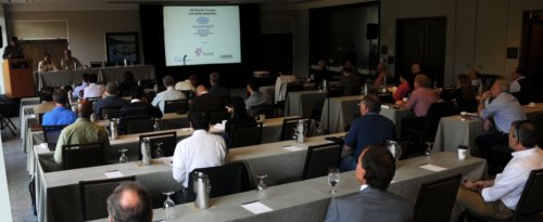
I am in Avon, Colorado, this week attending the SEG IQ Earth Forum. IQ (integrative and quantitative) Earth is a new SEG committee formed in reponse to a $1M monetary donation by Statoil to build a publicly available, industrial strength dataset for the petroleum community. In addition to hosting a standard conference format of podiums and Q and A's, the SEG is using the forum to ask delegates for opinions on how to run the committee. There are 12 people in attendance from consulting & software firms, 11 from service companies, 13 who work for operators, and 7 from SEG and academia. There's lively discussionafter each presentation, which has twice been cut short by adherence to the all important 2 hour lunch break. That's a shame. I wish the energy was left to linger. Here is a recap of the talks that have stood out for me so far:

Yesterday, Peter Wang from WesternGeco presented 3 mini-talks in 20 minutes showcasing novel treatments of uncertainty. In the first talk he did a stochastic map migration of 500 equally probable anisotropic velocity models that translated a fault plane within a 800 foot lateral uncertainty corridor. The result was even more startling on structure maps. Picking a single horizon or fault is wrong, and he showed by how much. Secondly, he showed a stocastic inversion using core, logs and seismic. He again showed the results of hundreds of non-unique but equally probable inversion realizations, each exactly fit the well logs. His point: one solution isn't enough. Only when we compute the range of possible answers can we quantify risk and capture our unknowns. Third, he showed an example from a North American resource shale, a setting where seismic methods are routinely under-utilized, and ironically, a setting where 70% of the production comes from less than 30% of the completed intervals. The geomechanical facies classification showed compelling frac barriers and non reservoir classes, coupled to an all-important error cube, showing the probability of each classification, the confidence of the method.

Ron Masters, from a software company called Headwave, presented a pre-recorded video demonstration of his software in action. Applause goes to him for a pseudo-interactive presentation. He used horizons as a boundary for scuplting away peripheral data for 3D AVO visualizations. He demostrated the technique of rotating a color wheel in the intercept-gradient domain, such that any and all linear combinations of AVO parameters can be mapped to a particular hue. No more need for hard polygons. Instead, with gradational crossplot color classes, the AVO signal doesn't get suddenly clipped out, unless there is a real change in fluid and lithology effects. Exposing AVO gathers in this interactive environment guards against imposing false distinctions that aren’t really there. 

The session today consisted of five talks from WesternGeco / Schlumberger, a powerhouse of technology who stepped up to show their heft. Their full occupancy of the podium today, gives a new meaning to the rhyming quip; all-day Schlumberger. Despite having the bias of an internal company conference, it was still very entertaining, and informative. 

Andy Hawthorn showed how seismic images can be re-migrated around the borehole (almost) in real time by taking velocity measurements while drilling. The new measurements help drillers adjust trajectories and mud weights entering hazardous high pressure which has remarkable safety and cost benefits. He showed a case where a fault was repositioned by 1000 vertical feet; huge implications for wellbore stability, placing casing shoes, and other such mechanical considerations. His premise is that the only problem worth our attention is the following: it is expensive to drill and produce wells. Science should not be done for the sake of it; but to build usable models for drillers. 

In a characteristically enthusiastic talk, Ran Bachrach showed how he incorporated a compacting shale anisotropic rock physics model with borehole temperature and porosity measurements to expedite empirical hypothesis testing of imaging conditions. His talk, like many before him throughout the Forum, touched on the notion of generating many solutions, as fast as possible. Asking questions of the data, and being able to iterate. 

At the end of the first day, Peter Wang stepped boldy back to the to the microphone while others has started packing their bags, getting ready to leave the room. He commented that what an "integrated and quantitative" earth model desperately needs are financial models and simulations. They are what drive this industry; making money. As scientists and technologists we must work harder to demonstrate the cost savings and value of these techniques. We aren't getting the word out fast enough, and we aren't as relevant as we could be. It's time to make the economic case clear.

Shooting into the dark

Part of what makes uncertainty such a slippery subject is that it conflates several concepts that are better kept apart: precision, accuracy, and repeatability. People often mention the first two, less often the third.

It's clear that precision and accuracy are different things. If someone's shooting at you, for instance, it's better that they are inaccurate but precise so that every bullet whizzes exactly 1 metre over your head. But, though the idea of one-off repeatability is built in to the concept of multiple 'readings', scientists often repeat experiments and this wholesale repeatability also needs to be captured. Hence the third drawing. 

One of the things I really like in Peter Copeland's book Communicating Rocks is the accuracy-precision-repeatability figure (here's my review). He captured this concept very nicely, and gives a good description too. There are two weaknesses though, I think, in these classic target figures. First, they portray two dimensions (spatial, in this case), when really each measurement we make is on a single axis. So I tried re-drawing the figure, but on one axis:

The second thing that bothers me is that there is an implied 'correct answer'—the middle of the target. This seems reasonable: we are trying to measure some external reality, after all. The problem is that when we make our measurements, we do not know where the middle of the target is. We are blind.

If we don't know where the bullseye is, we cannot tell the difference between precise and imprecise. But if we don't know the size of the bullseye, we also do not know how accurate we are, or how repeatable our experiments are. Both of these things are entirely relative to the nature of the target. 

What can we do? Sound statistical methods can help us, but most of us don't know what we're doing with statistics (be honest). Do we just need more data? No. More expensive analysis equipment? No.

No, none of this will help. You cannot beat uncertainty. You just have to deal with it.

This is based on an article of mine in the February issue of the CSEG Recorder. Rather woolly, even for me, it's the beginning of a thought experiment about doing a better job dealing with uncertainty. See Hall, M (2012). Do you know what you think you know? CSEG Recorder, February 2012. Online in May. Figures are here.