Unweaving the rainbow

Last week at the Canada GeoConvention in Calgary I gave a slightly silly talk on colourmaps with Matteo Niccoli. It was the longest, funnest, and least fruitful piece of research I think I've ever embarked upon. And that's saying something.

Freeing data from figures

It all started at the Unsession we ran at the GeoConvention in 2013. We asked a roomful of geoscientists, 'What are the biggest unsolved problems in petroleum geoscience?'. The list we generated was topped by Free the data, and that one topic alone has inspired several projects, including this one. 

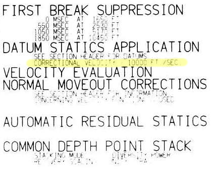
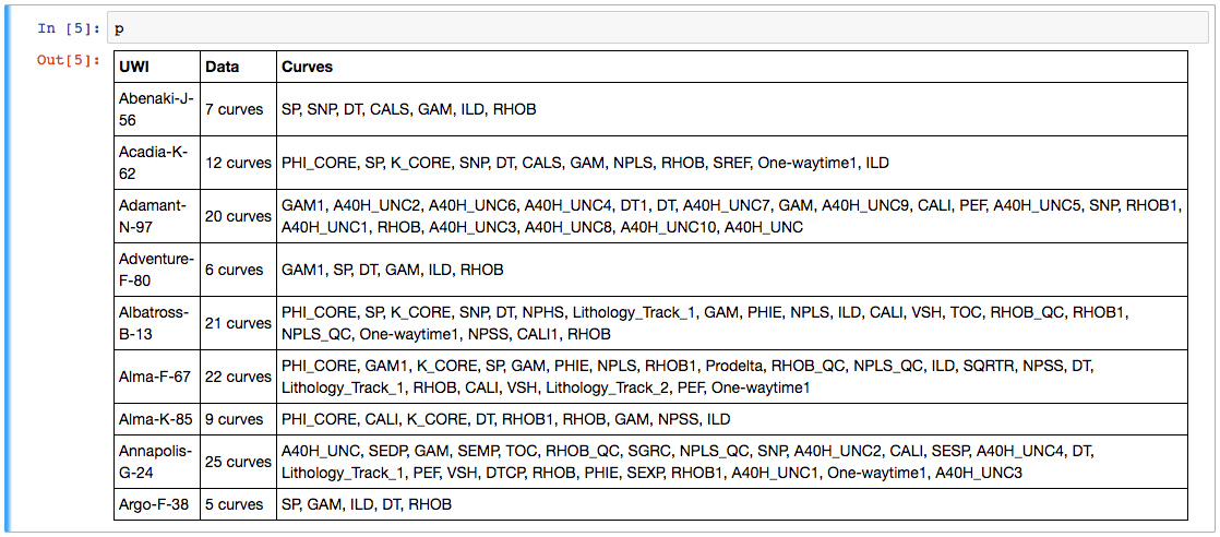
Our goal: recover digital data from any pseudocoloured scientific image, without prior knowledge of the colourmap.

I subsequently proferred this challenge at the 2015 Geophysics Hackathon in New Orleans, and a team from Colorado School of Mines took it on. Their first step was to plot a pseudocoloured image in (red, green blue) space, which reveals the colourmap and brings you tantalizingly close to retrieving the data. Or so it seems...

Here's our talk:

x lines of Python: machine learning

You might have noticed that our web address has changed to agilescientific.com, reflecting our continuing journey as a company. Links and emails to agilegeoscience.com will redirect for the foreseeable future, but if you have bookmarks or other links, you might want to change them. If you find anything that's broken, we'd love it if you could let us know.

---

Artificial intelligence in 10 lines of Python? Is this really the world we live in? Yes. Yes it is.

After reminding you about the SEG machine learning contest just before Christmas, I thought I could show you how you train a model in a supervised learning problem, then use it to make predictions on unseen data. So we'll just break a simple contest entry down into ten easy steps (note that you could do this on anything, doesn't have to be this problem). 

A machine learning primer

Before we start, let's review quickly what a machine learning problem looks like, and introduct a bit of jargon. To begin, we have a dataset (e.g. the 'Old' well in the diagram below). This consists of records, called instances. In this problem, each instance is a depth location. Each instance is a feature vector: a row vector comprising attributes or features, which in our case are wireline log values for GR, ILD, and so on. Each feature vector is a row in a matrix we conventionally call \(X\). Associated with each instance is some target label — the thing we want to predict — which is a continuous quantity in a regression problem, discrete in a classification problem. The vector of labels is usually called \(y\). In the problem below, the labels are integers representing 9 different facies.

View fullsize

You can read much more about the dataset I'm using in Brendon Hall's tutorial (The Leading Edge, October 2016).

The ten steps to glory

Well, maybe not glory, but something. A prediction of facies at two wells, based on measurements made at 10 other wells. You can follow along in the notebook, but all the highlights are included here. We start by loading the data into a 'dataframe', which you can think of like a spreadsheet:

Now we specify the features we want to use, and make the matrix \(X\) and label vector \(y\):

  features = ['GR', 'ILD_log10', 'DeltaPHI', 'PHIND', 'PE']
  X = df[features].values
  y = df.Facies.values

Since this dataset is all we have, we'd like to set aside some data to test our model on. The library we're using, scikit-learn, has functions to do this sort of thing; by default, it'll split \(X\) and \(y\) into train and test datasets, with 25% of the data going into the test part:

  X_train, X_test, y_train, y_test = train_test_split(X, y)

Now we're ready to choose a model, instantiate it (with some parameters if we want), and train the model (i.e. 'fit' the data). I am calling the trained model augur, because I like that word.

  from sklearn.ensemble import ExtraTreesClassifier
  model = ExtraTreesClassifier()
  augur = model.fit(X_train, y_train)

Now we're ready to take the part of the dataset we reserved for validation, X_test, and predict its labels. Then we can compare those with the known labels, y_test, to see how well we did:

  y_pred = augur.predict(X_test)

We can get a quick idea of the quality of prediction with sklearn.metrics.accuracy_score(y_test, y_pred), but it's more interesting to look at the classification report, which shows us the precision and recall for each class, along with their harmonic mean, the F1 score:

  from sklearn.metrics import classification_report
  print(classification_report(y_test, y_pred))

Each row is a facies (facies 1, facies 2, etc.). The support is the number of instances representing that label. The key number here is 0.63 — we can regard this as an expression of the accuracy of our prediction. If that sounds low to you, I encourage you to enter the machine learning contest! If it sounds high, that's because it is — it's much too high. In fact, the instances of our dataset are not independent: they are spatially correlated (in depth). It would be smarter not to remove some random samples for validation, but to reserve entire wells. After all, this is how we typically collect subsurface data: one well at a time.

But now we're getting into the weeds of data science. I'll let you venture in there on your own...

Burning the surface onto the subsurface

Previously, I described a few of the reasons why we don't get a clean ground surface event on land seismic data like we do the water-bottom in marine seismic. In land data, the worst part of the image is right at the surface. But ground level is not just tricky to see, it's impossible to see. Since the vibe truck is on the ground, there's no reflection from that surface. Even if there was some kind of event there, processors apply a magic eraser to the top of the section — the mute — to erase the early arrivals. So it's not possible to see the ground in land data, and you can't pick what isn't there.  

But I still want to know where the ground is. Why can't we slap a ground-level seismic 'reflection' event on the section? 

What you need

We need the ground level, which is in depth of course, in the time domain of the seismic section. To compute this, let's call it \(t_\mathrm{G}\), we need three pieces of information at every trace location: the ground elevation \(G\), the seismic reference datum (SRD) which I'll call \(D\), and the replacement velocity \(V_\mathrm{r}\). 

$$ t_\mathrm{G} = \frac{2 (G - D)}{V_\mathrm{r}} $$

Ground elevation.  If you're lucky, you'll be able to find the ground elevation corresponding to each trace stored in the trace headers. Ground elevation might be located in bytes 41-44 or 45-48 of the trace header, which correspond to the receiver group elevation and the surface elevation of the source, respectively. These should be the same for a stacked trace, but as with any meta-data to do with SEGY, this info could be hiding somewhere else, or missing altogether. And if you're that unlucky, you might have to comb through processing reports for the missing information. If you are even more unlucky (as I was in this example), you won't have any kind of processing report to fall back on and you'll have to concoct something else. In the accompanying Jupyter notebook, I resorted to interpolating a digitized elevation profile from a JPEG plot of the seismic line. So if you're all out of options, you might find refuge in those legacy plots! 

This profile is particularly wonky, because the seismic reference datum (red) is not the same across the profile

Seismic reference datum. And to make life yet more complicated, the seismic reference datum is not flat across the profile. It goes downhill and then flattens out (red line below). Don't ask me what the advantages are of processing data to a variable datum, but whatever they are, I hope they offset the disadvantages of all-to-easily mistaking the datum to be flat.

The replacement velocity is given in the sidelabel of the raster image online (shown right). It's 10 000 ft/sec, or 3048 m/s. 

Byte locations 53-56 and 57-60 are the standard trace header placeholders reserved for holding the datum elevation at the receiver group and the datum elevation at source. Again, for a stacked trace, these should be the same value. If these fields are zeros, then check the fields of the Trace Header Extension. If they turn up empty, and if the datum is horizontal, it might be listed in the file's text header. 

Convert elevation to time

By definition, the seismic reference datum is horizontal in the time-domain (red line below). Notice how the ground elevation – in the time domain – plots mostly as negative values (before) time zero. In other words, most of the ground is being cut-off by the top of the section. So, if we want to see it, we need to shift everything down into the field of view. Conceptually, this means adjusting the seismic reference datum so it floats entirely above the ground-level. Computationally, we can achieve this easily enough by padding the top of the data with zeros.

A time-domain representation of the ground-level along the seismic profile. The surface of the earth extends above the start of the seismic data for most of the locations along the profile. 

Make the ground a pickable event

As a final bit of post-processing, we could actually burn the ground-level into the data as a sort of synthetic seismic event. The reason I like this concept is that it alleviates the need to dig up old-processing reports, puzzle over missing header data, or worse, maintain and munge external text files containing elevation information. I say, let's make it self-contained. Let's put it directly into the data so that it can be treated like any other seismic reflection. Why would I do this?

• You can see where there might be fold, velocity or other issues related to topography.
• You can immediately see the polarity of the data. 
• You could use the bandwidth of the data to make the pseudo-reflector, giving a visual hint to the interpreter.
• Keeping track of amplitude adjustments and phase rotations would be self-documenting and reversible.
• you could autotrack it to get a topographic map (or just get this from the processor).
• It looks cool!

Seismic profile with ground level SYNTHETICALLY SLAPPED ON TOP.  Bandlimited, of course, so you can Autotrack till your hearts content!

I've deliberately constructed a band-limited reflection, opposed to placing a sharp spike at ground-level. The problem with a spike is that it has infinite bandwidth. It contains higher frequencies than the image, so as Carl Reine commented on that last post, that might not play nice with seismic attributes. Also, there's the problem of selecting an amplitude value to assign to the spike: we don't want to introduce amplitudes that are ridiculously out of range of the existing data.  

The whole image

I hereby propose that this synthetic ground level trick adopted as the new standard for any land seismic processing and interpretation. The great thing is, it can be done just as easily by interpreters and seismic data technologists, as by the processing companies that create the rest of the image. I realize we're adding stuff to the data that isn't actually signal. We do non-real things to signals all the time. The question is, do the benefits outweigh the artificiality?

Here's the view of the entire section:

The whole section, ground level included.

The details of this exercise can be found in the this Jupyter Notebook.

References

The seismic is line 36_77_PR from the USGS data repository.

SEG Y rev 2 Data Exchange Format. SEG Technical Standards Committee. Draft 2.0, January, 2015. 

Where is the ground?

This is the upper portion of a land seismic profile in Alaska. Can you pick a horizon where the ground surface is? Have a go at pickthis.io.

Pick the Ground surface at the top of the seismic section at pickthis.io.

Picking the ground surface on land-based seismic data is not straightforward. Picking the seafloor reflection on marine data, on the other hand, is usually a piece of cake, a warm-up pick. You can often auto-track the whole thing with a few seeds.

Seafloor reflection on Penobscot 3D survey, offshore Nova Scotia. from Matt's tutorial in the April 2016 The Leading Edge, The function of interpolation.

Why aren't interpreters more nervous that we don't know exactly where the surface of the earth is? I'm sure I'm not the only one that would like to have this information while interpreting. Wouldn't it be great if land seismic were more like marine?

Treacherously Jagged TopographY or Near-Surface processing ArtifactS?

If you're new to land-based seismic data, you might notice that there isn't a nice pickable event across the top of the section like we find in marine seismic data. Shot noise at the surface has been muted (deleted) in processing, and the low fold produces an unclean, jagged look at the top of the section. Additionally, the top of the section, time-zero — the seismic reference datum — usually floats somewhere above the land surface — and we can't know where that is unless it can be found in the file header, or looked up in the processing report.

The seismic reference datum, at a two-way time of zero seconds on seismic data, is typically set at mean sea level for offshore data. For land data, it is usually chosen to 'float' above the land surface.

Reframing the question

This challenge is a bit of a trick question. It begs the viewer to recognize that the seemingly simple task of mapping the ground level on a land seismic section is actually a rudimentary velocity modeling or depth conversion exercise in itself. Wouldn't it be nice to have the ground surface expressed as pickable seismic event? Shouldn't we have it always in our images? Baked into our data, so to speak, such that we've always got an unambiguous pick? In the next post, I'll illustrate what I mean and show what's involved in putting it in. 

In the meantime, I challenge you to pick where you think the (currently absent) ground surface is on this profile, so in the next post we can see how well you did.

Welly to the wescue

I apologize for the widiculous title.

Last week I described some headaches I was having with well data, and I introduced welly, an open source Python tool that we've built to help cure the migraine. The first versions of welly were built — along with the first versions of striplog — for the Nova Scotia Department of Energy, to help with their various data wrangling efforts.

Aside — all software projects funded by government should in principle be open source.

Today we're using welly to get data out of LAS files and into so-called feature vectors for a machine learning project we're doing for Canstrat (kudos to Canstrat for their support for open source software!). In our case, the features are wireline log measurements. The workflow looks something like this:

1. Read LAS files into a welly 'project', which contains all the wells. This bit depends on lasio.
2. Check what curves we have with the project table I showed you on Thursday.
3. Check curve quality by passing a test suite to the project, and making a quality table (see below).
4. Fix problems with curves with whatever tricks you like. I'm not sure how to automate this.
5. Export as the X matrix, all ready for the machine learning task.

Let's look at these key steps as Python code.

1. Read LAS files

from welly import Project
p = Project.from_las('data/*.las')

2. Check what curves we have

Now we have a project full of wells and can easily make the table we saw last week. This time we'll use aliases to simplify things a bit — this trick allows us to refer to all GR curves as 'Gamma', so for a given well, welly will take the first curve it finds in the list of alternatives we give it. We'll also pass a list of the curves (called keys here) we are interested in:

The project table. The name of the curve selected for each alias is selected. The mean and units of each curve are shown as a quick QC. A couple of those RHOB curves definitely look dodgy, and they turned out to be DRHO correction curves.

3. Check curve quality

Now we have to define a suite of tests. Lists of test to run on each curve are held in a Python data structure called a dictionary. As well as tests for specific curves, there are two special test lists: Each and All, which are run on each curve encountered, and on all curves together, respectively. (The latter is required to, for example, compare the curves to each other to look for duplicates). The welly module quality contains some predefined tests, but you can also define your own test functions — these functions take a curve as input, and return either True (for a test pass) for False.

import welly.quality as qty
tests = {
    'All': [qty.no_similarities],
    'Each': [qty.no_monotonic],
    'Gamma': [
        qty.all_positive,
        qty.mean_between(10, 100),
    ],
    'Density': [qty.mean_between(1000,3000)],
    'Sonic': [qty.mean_between(180, 400)],
    }

html = p.curve_table_html(keys=keys, alias=alias, tests=tests)
HTML(html)

the green dot means that all tests passed for that curve. Orange means some tests failed. If all tests fail, the dot is red. The quality score shows a normalized score for all the tests on that well. In this case, RHOB and DT are failing the 'mean_between' test because they have Imperial units.

4. Fix problems

Now we can fix any problems. This part is not yet automated, so it's a fairly hands-on process. Here's a very high-level example of how I fix one issue, just as an example:

def fix_negs(c):
    c[c < 0] = np.nan
    return c

# Glossing over some details, we give a mnemonic, a test
# to apply, and the function to apply if the test fails.
fix_curve_if_bad('GAM', qty.all_positive, fix_negs)

What I like about this workflow is that the code itself is the documentation. Everything is fully reproducible: load the data, apply some tests, fix some problems, and export or process the data. There's no need for intermediate files called things like DT_MATT_EDIT or RHOB_DESPIKE_FINAL_DELETEME. The workflow is completely self-contained.

5. Export

The data can now be exported as a matrix, specifying a depth step that all data will be interpolated to:

X, _ = p.data_as_matrix(X_keys=keys, step=0.1, alias=alias)

That's it. We end up with a 2D array of log values that will go straight into, say, scikit-learn*. I've omitted here the process of loading the Canstrat data and exporting that, because it's a bit more involved. I will try to look at that part in a future post. For now, I hope this is useful to someone. If you'd like to collaborate on this project in the future — you know where to find us.

* For more on scikit-learn, don't miss Brendon Hall's tutorial in October's Leading Edge.

---

I'm happy to let you know that agilegeoscience.com and agilelibre.com are now served over HTTPS — so connections are private and secure by default. This is just a matter of principle for the Web, and we go to great pains to ensure our web apps modelr.io and pickthis.io are served over HTTPS. Find out more about SSL from DigiCert, the provider of Squarespace's (and Agile's) certs, which are implemented with the help of the non-profit Let's Encrypt, who we use and support with dollars.

Well data woes

I probably shouldn't be telling you this, but we've built a little tool for wrangling well data. I wanted to mention it, becase it's doing some really useful things for us — and maybe it can help you too. But I probably shouldn't because it's far from stable and we're messing with it every day.

But hey, what software doesn't have a few or several or loads of bugs?

Buggy data?

It's not just software that's buggy. Data is as buggy as heck, and subsurface data is, I assert, the buggiest data of all. Give units or datums or coordinate reference systems or filenames or standards or basically anything at all a chance to get corrupted in cryptic ways, and they take it. Twice if possible.

By way of example, we got a package of 10 wells recently. It came from a "data management" company. There are issues... Here are some of them:

• All of the latitude and longitude data were in the wrong header fields. No coordinate reference system in sight anywhere. This is normal of course, and the only real side-effect is that YOU HAVE NO IDEA WHERE THE WELL IS.
• Header chaos aside, the files were non-standard LAS sort-of-2.0 format, because tops had been added in their own little completely illegal section. But the LAS specification has a section for stuff like this (it's called OTHER in LAS 2.0).
• Half the porosity curves had units of v/v, and half %. No big deal...
• ...but a different half of the porosity curves were actually v/v. Nice.
• One of the porosity curves couldn't make its mind up and changed scale halfway down. I am not making this up.
• Several of the curves were repeated with other names, e.g. GR and GAM, DT and AC. Always good to have a spare, if only you knew if or how they were different. Our tool curvenam.es tries to help with this, but it's far from perfect.
• One well's RHOB curve was actually the PEF curve. I can't even...

The remarkable thing is not really that I have this headache. It's that I expected it. But this time, I was out of paracetamol.

Cards on the table

Our tool welly, which I stress is very much still in development, tries to simplify the process of wrangling data like this. It has a project object for collecting a lot of wells into a single data structure, so we can get a nice overview of everything: 

View fullsize

Click to enlarge.

Our goal is to include these curves in the training data for a machine learning task to predict lithology from well logs. The trained model can make really good lithology predictions... if we start with non-terrible data. Next time I'll tell you more about how welly has been helping us get from this chaos to non-terrible data.

x lines of Python: read and write SEG-Y

Reading SEG-Y files comes up a lot in the geophysicist's workflow. Writing, less often, but it does come up occasionally. As long as we're mostly concerned with trace data and not location, both of these tasks can be fairly easily accomplished with ObsPy. 

Today we'll load some seismic, compute an attribute on it, and save a new SEG-Y, in 10 lines of Python.

---

ObsPy is a rare thing. It demonstrates what a research group can accomplish with a little planning and a lot of perseverance (cf my whinging earlier this year about certain consortiums in our field). It's an open source Python package from the geophysicists at the University of Munich — Karl Bernhard Zoeppritz studied there for a while, so you know it's legit. The tool serves their research in earthquake and global seismology needs, and also happens to handle SEG-Y files quite nicely.

Aside: I think SixtyNorth's segpy is actually the way to go for reading and writing SEG-Y; ObsPy is probably overkill for most applications — it's about 80 times the size for one thing. I just happen to be familiar with it and it's super easy to install: conda install obspy. So, since minimalism is kind of the point here, look out for a future x lines of Python using that library.

The sentences

As before, we'd like to express the process in just a few sentences of plain English. Assuming we just want to read the data into a NumPy array, look at it, do something to it, and write a new file, here's what we're doing:

1. Read (or really index) the file as an ObsPy Stream object.
2. Stack (in the NumPy sense) the Trace objects into a single NumPy array. We have data!
3. Get the 99th percentile of the amplitudes to make plotting easier.
4. Plot the data so we can see it.
5. Get the sample interval of the data from a trace header.
6. Compute the similarity attribute using our library bruges.
7. Make a new Stream object to hold the outbound data.
8. Add a Stats object, which holds the header, and recycle some header info.
9. Append info about our data to the header.
10. Write a new SEG-Y file with our computed data in it!

There's a bit more in the Jupyter Notebook (examining the file and trace headers, for example, and a few more plots) which, remember, you can run right in your browser! You don't need to install a thing. Please give it a look! Quick tip: Just keep hitting Shift+Enter to run the cells.

If you like this sort of thing, and are planning to be at the SEG Annual Meeting in Dallas next month, you might like to know that we'll be teaching our Creative Geocomputing class there. It's basically two days of this sort of thing, only with friends to learn with and us to help. Come and learn some new skills!

---

The seismic data used in this post is from the NPRA seismic repository of the USGS. The data is in the public domain.

x lines of Python: synthetic wedge model

Welcome to a new blog series! Like the A to Z and the Great Geophysicists, I expect it will be sporadic and unpredictable, but I know you enjoys life's little nonlinearities as much as I.

The idea with this one — x lines of Python — is to share small geoscience workflows in x lines or fewer. I'm not sure about the value of x, but I think 10 seems reasonable for most tasks. If x > 10 then the task may have been too big... If x < 5 then it was probably too small.

Python developer Raymond Hettinger says that each line of code should be equivalent to a sentence... so let's say that that's the measure of what's OK to put in a single line. 

Synthetic wedge model

To kick things off, follow this link to a live Jupyter Notebook environment showing how you can make a simple synthetic three-rock wedge model in only 9 lines of code.

The sentences represented by the code that made the data in these images are:

1. Set up the size of the model.
2. Make the slanty bit, with 1's in the wedge and 2's in the base.
3. Add the top of the model as 0; these numbers will turn into rocks.
4. Define the velocity and density of rocks 0 to 2.
5. Distribute those properties through the model.
6. Calculate the acoustic impedance everywhere.
7. Calculate the reflection coefficients in the model.
8. Make a Ricker wavelet.
9. Convolve the wavelet with the reflection coefficients.

Your turn!

All of the notebooks we share in this series will be hosted on mybinder.org. I'm excited about this because it means you can run and edit them live, without installing anything at all. Give it a go right now.

You can see them on GitHub too, and fork or clone them from there. Note that if you look at the notebook for this post on GitHub, you'll be able to view it, but not change or run code unless you get everything running on your own machine. (To do that, you can more or less follow the instructions in my User Guide to the TLE tutorials).

Please do take this notion of x as 'par' as a challenge. If you'd like to try to shoot under par, please do — and share your efforts. Code golf is a fun way to learn better coding habits. (And maybe some bad ones.) There is a good chance I will shoot some bogies on this course.

We will certainly take requests too — what tasks would you like to see in x lines of Python?

Helpful horizons

Ah, the smell of a new seismic interpretation project. All those traces, all that geology — perhaps unseen by humans or indeed any multicellular organism at all since the Triassic. The temptation is to Just Start Interpreting, why, you could have a map by lunchtime tomorrow! But wait. There are some things to do first.

Once I've made sure all is present and correct (see How to QC a seismic volume), I spend a bit of time making some helpful horizons... 

• The surface. One of the fundamental horizons, the seafloor or ground surface is a must-have. You may have received it from the processor (did you ask for it?) or it may be hidden in the SEG-Y headers — ask whoever received or loaded the data. If not, ground elevation is usually easy enough to get from your friendly GIS guru. If you have to interpret the seafloor, at least it should autotrack quite well.
• Seafloor multiple model. In marine data, I always make a seafloor multiple model — just multiply the seafloor pick by 2. This will help you make sense of any anomalous reflectors or amplitudes at that two-way time. Maybe make a 3× version too if things look really bad. Remember, the 2× multiple will be reverse polarity.
• Other multiples. You can model the surface multiple of any strong reflectors with the same arithmetic — but the chances are that any residual multiple energy is quite subtle. You may want to seek help modeling them properly, once you have a 3D velocity model.

View fullsize

A 2D seismic dataset with some of the suggested helpful horizons. Please see the footnote about this dataset. Click the image to enlarge.

• Water depth markers. I like to make flat horizons* at important water depths, eg shelf edge (usually about 100–200 m), plus 1000 m, 2000 m, etc. This mainly helps to keep track of where you are, and also to think about prospectivity, accessibility, well cost, etc. You only want these to exist in the water, so delete them anywhere they are deeper than the seafloor horizon. Your software should have an easy way to implement a simple model for time t in ms, given depth d in m and velocity** V in m/s, e.g.

$$ t = \frac{2000 d}{V} \approx \frac{2000 d}{1490} \qquad \qquad \mathrm{e.g.}\ \frac{2000 \times 1000}{1490} = 1342\ \mathrm{ms} $$

• Hydrate stability zone. In marine data and in the Arctic you may want to model the bottom of the gas hydrate stability zone (GHSZ) to help interpret bottom-simulating reflectors, or BSRs. I usually do this by scanning the literature for reports of BSRs in the area, or data on hydrate encounters in wells. In the figure above, I just used the seafloor plus 400 ms. If you want to try for more precision, Bale et al. (2014) provided several models for computing the position of the GHSZ — thank you to Murray Hoggett at Birmingham for that tip.
• Fold. It's very useful to be able to see seismic fold on a map along with your data, so I like to load fold maps at some strategic depths or, better yet, load the entire fold volume. That way you can check that anomalies (especially semblance) don't have a simple, non-geological explanation. 
• Gravity and magnetics. These datasets are often readily available. You will have to shift and scale them to some sensible numbers, either at the top or the bottom of your sections. Gravity can be especially useful for interpreting rifted margins. 
• Important boundaries. Your software may display these for you, but if not, you can fake it. Simply make a horizon that only exists within the polygon — a lease boundary perhaps — by interpolating within a polygon. Make this horizon flat and deep (deeper than the seismic), then merge it with a horizon that is flat and shallow (–1 ms, or anything shallower than the seismic). You should end up with almost-vertical lines at the edges of the feature.
• Section headings. I like to organize horizons into groups — stratigraphy, attributes, models, markers, etc. I make empty horizons to act only as headings so I can see at a glance what's going on. Whether you need do this, and how you achieve it, depends on your software.

Most of these horizons don't take long to make, and I promise you'll find uses for them throughout the interpretation project. 

If you have other helpful horizon hacks, I'd love to hear about them — put your favourites in the comments. 

---

Footnotes

* It's not always obvious how to make a flat horizon. A quick way is to take some ubiquitous horizon — the seafloor maybe — and multiply it by zero.

** The velocity of sound in seawater is not a simple subject. If you want to be precise about it, you can try this online calculator, or implement the equations yourself.

The 2D seismic dataset shown is from the Laurentian Basin, offshore Newfoundland. The dataset is copyright of Natural Resources Canada, and subject to the Open Government License – Canada. You can download it from the OpendTect Open Seismic Repository. The cultural boundary and gravity data is fictitious — I made them up for the purposes of illustration.

References

Bale, Sean, Tiago M. Alves, Gregory F. Moore (2014). Distribution of gas hydrates on continental margins by means of a mathematical envelope: A method applied to the interpretation of 3D seismic data. Geochem. Geophys. Geosyst. 15, 52–68, doi:10.1002/2013GC004938. Note: the equations are in the Supporting Information.

White magic: calibrating seismic attributes

This post is part of a series on seismic attributes; the previous posts were...

1. An attribute analysis primer
2. Attribute analysis and statistics

---

Last time, I hinted that there might be a often-overlooked step in attribute analysis:

Calibration is a gaping void in many published workflows. How can we move past "that red blob looks like a point bar so I drew a line around it in PowerPoint" to "there's a 70% chance of finding reservoir quality sand at that location"?

Why is this step such a 'gaping void'? A few reasons:

• It's fun playing with attributes, and you can make hundreds without a second thought. Some of them look pretty interesting, geological even. "That looks geological" is, however, not an attribute calibration technique. You have to prove it.
• Nobody will be around when we find out the answer. There's a good chance that well will never be drilled, but when it is, you'll be on a different project, in a different company, or have left the industry altogether and be running a kayak rental business in Belize.
• The bar is rather low. The fact that many published examples of attribute analysis include no proof at all, just a lot of maps with convincing-looking polygons on them, and claims of 'better reservoir quality over here'. 

This is getting discouraging. Let's look at an example. Now, it's hard to present this without seeming over-critical, but I know these gentlemen can handle it, and this was only a magazine article, so we needn't make too much of it. But it illustrates the sort of thing I'm talking about, so here goes.

Quoting from Chopra & Marfurt (AAPG Explorer, April 2014), edited slightly for brevity:

While coherence shows the edges of the channel, it gives little indication of the heterogeneity or uniformity of the channel fill. Notice the clear definition of this channel on the [texture attribute — homogeneity].

We interpret [the] low homogeneity feature [...] to be a point bar in the middle of the incised valley (green arrow). This internal architecture was not delineated by coherence.

A nice story, making two claims:

1. The attribute incompletely represents the internal architecture of the channel.
2. The labeled feature on the texture attribute is a point bar.

I know explorers have to be optimists, and geoscience is all about interpretation, but as scientists we must be skeptical optimists. Claims like this are nice hypotheses, but you have to take the cue: go off and prove them. Remember confirmation bias, and Feynman's words:

The first principle is that you must not fool yourself — and you are the easiest person to fool.

The twin powers

Making geological predictions with seismic attribute analysis requires two related workflows:

1. Forward modeling — the best way to tune your intuition is to make a cartoonish model of the earth (2D, isotropic, homogeneous lithologies) and perform a simplified seismic experiment on it (convolutional, primaries only, noise-free). Then you can compare attribute behaviour to the known model.
2. Calibration — you are looking for an explicit, quantitative relationship between a physical property you care about (porosity, lithology, fluid type, or whatever) and a seismic attribute. A common way to show this is with a cross-plot of the seismic amplitude against the physical property.

When these foundations are not there, we can be sure that one or more bad things will happen:

• The relationship produces a lot of type I errors (false positives).
• It produces a lot of type II error (false negatives).
• It works at some wells and not at others.
• You can't reproduce it with a forward model.
• You can't explain it with physics.

As the industry shrivels and questions — as usual — the need for science and scientists, we have to become more stringent, more skeptical, and more rigorous. Doing anything else feeds the confirmation bias of the non-scientific continent. Because it says, loud and clear: geoscience is black magic.

---

The image is part of the figure from Chopra, S and K Marfurt (2014). Extracting information from texture attributes. AAPG Explorer, April 2014. It is copyright of the Authors and AAPG.