SciPy will eat the world... in a good way

We're at the SciPy 2014 conference in Austin, the big giant meetup for everyone into scientific Python.

One surprising thing so far is the breadth of science and computing in play, from astronomy to zoology, and from AI to zero-based indexing. It shouldn't have been surprising, as SciPy.org hints at the variety:

There's really nothing you can't do in the scientific Python ecosystem, but this isn't why SciPy will soon be everywhere in science, including geophysics and even geology. I think the reason is IPython Notebook, and new web-friendly ways to present data, directly from the computing environment to the web — where anyone can see it, share it, interact with it, and even build on it in their own work.

Teaching STEM

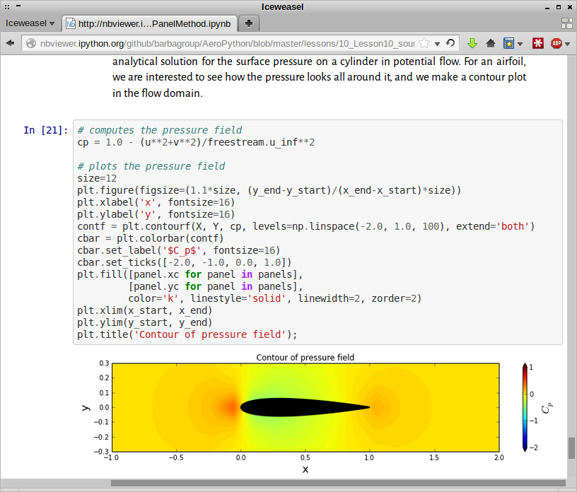
In Tuesday's keynote, Lorena Barba, an uber-prof of engineering at The George Washington University, called IPython Notebook the killer app for teaching in the STEM fields. She has built two amazing courses in Notebook: 12 Steps to Navier–Stokes and AeroPython (right), and more are on the way. Soon, perhaps through Jupyter CoLaboratory (launching in alpha today), perhaps with the help of tools like Bokeh or mpld3, the web versions of these notebooks will be live and interactive. Python is already the new star of teaching computer science, web-friendly super-powers will continue to push this.

Let's be extra clear: if you are teaching geophysics using a proprietary tool like MATLAB, you are doing your students a disservice if you don't at least think hard about moving to Python. (There's a parallel argument for OpedTect over Petrel, but let's not get into that now.)

Reproducible and presentable

Can you imagine a day when geoscientists wield these data analysis tools with the same facility that they wield other interpretation software? With the same facility that scientists in other disciplines are already wielding them? I can, and I get excited thinking about how much easier it will be to collaborate with colleagues, document our workflows (for others and for our future selves), and write presentations and papers for others to read, interact with, and adapt for their own work.

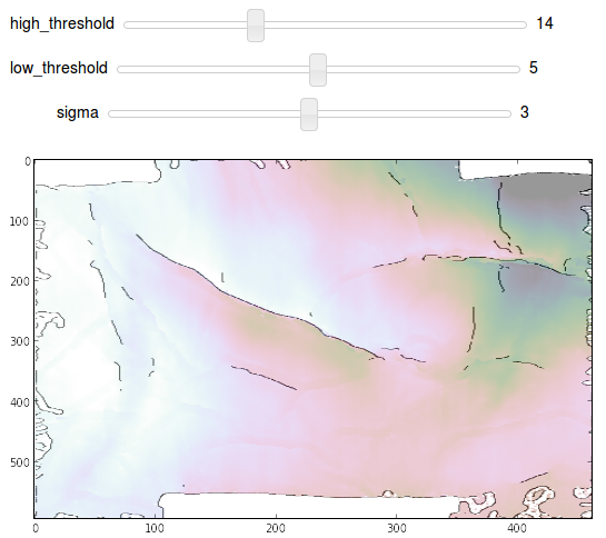
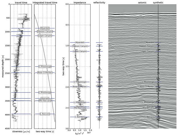
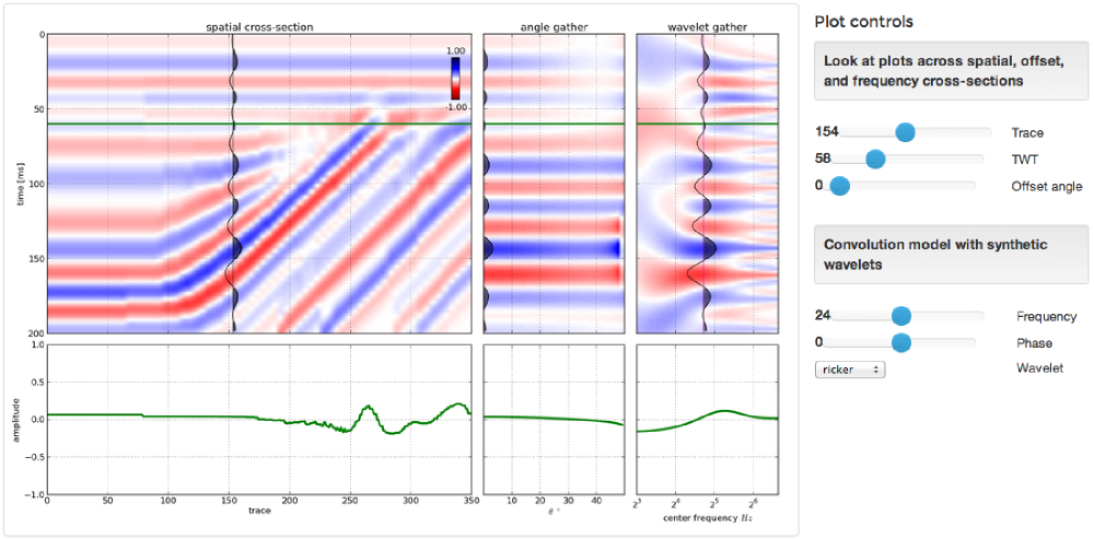
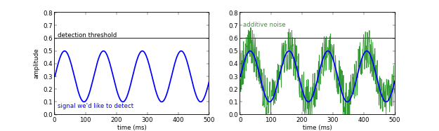
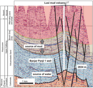
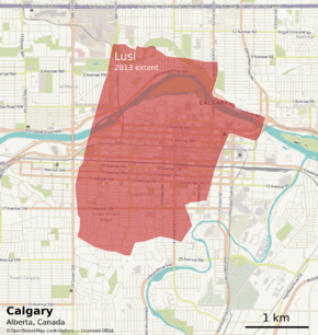
To whet your appetite, here's the sort of thing I mean (not interactive, but here's the code)...

If you agree that it's needed, I want to ask: What traditions or skill gaps are in the way of this happening? How can our community of scientists and engineers drive this change? If you disagree, I'd love to hear why.

Well tie calculus

As Matt wrote in March, he is editing a regular Tutorial column in SEG's The Leading Edge. I contributed the June edition, entitled Well-tie calculus. This is a brief synopsis only; if you have any questions about the workflow, or how to get started in Python, get in touch or come to my course.


Synthetic seismograms can be created by doing basic calculus on traveltime functions. Integrating slowness (the reciprocal of velocity) yields a time-depth relationship. Differentiating acoustic impedance (velocity times density) yields a reflectivity function along the borehole. In effect, the integral tells us where a rock interface is positioned in the time domain, whereas the derivative tells us how the seismic wavelet will be scaled.

This tutorial starts from nothing more than sonic and density well logs, and some seismic trace data (from the #opendata Penobscot dataset in dGB's awesome Open Seismic Repository). It steps through a simple well-tie workflow, showing every step in an IPython Notebook:

  1. Loading data with the brilliant LASReader
  2. Dealing with incomplete, noisy logs
  3. Computing the time-to-depth relationship
  4. Computing acoustic impedance and reflection coefficients
  5. Converting the logs to 2-way travel time
  6. Creating a Ricker wavelet
  7. Convolving the reflection coefficients with the wavelet to get a synthetic
  8. Making an awesome plot, like so...

Final thoughts

If you find yourself stretching or squeezing a time-depth relationship to make synthetic events align better with seismic events, take the time to compute the implied corrections to the well logs. Differentiate the new time-depth curve. How much have the interval velocities changed? Are the rock properties still reasonable? Synthetic seismograms should adhere to the simple laws of calculus — and not imply unphysical versions of the earth.


Matt is looking for tutorial ideas and offers to write them. Here are the author instructions. If you have an idea for something, please drop him a line.

Patents are slowing us down

I visited a geoscience consulting company in Houston recently. Various patent awards were proudly commemorated on the walls on little plaques. It's understandable: patents are difficult and expensive to get, and can be valuable to own. But recently I've started to think that patents are one of the big reasons why innovation in our industry happens at a snail's pace, in the words of Paul de Groot in our little book about geophysics. 

Have you ever read a patent? Go and have a read of US Patent 8670288, by Børre Bjerkholt of Schlumberger. I'll wait here.

What are they for?

It is more or less totally unreadable. And Google's rendering, even the garbled math, is much nicer than the USPTO's horror show. Either way, I think it's safe to assume that almost no-one will ever read it. Apart from anything else, it's written in lawyerspeak, and who wants to read that stuff?

Clearly patents aren't there to inform. So why are they there?

  • To defend against claims of infringement by others? This seems to be one of the main reasons technology companies are doing it.
  • To intimidate others into not trying to innovate or commercialize an innovation? With the possible unintended consequence of forcing competitors to avoid trouble by being more inventive.
  • To say to Wall Street (or whoever), "we mean business"? Patents are valuable: the median per-patent price paid in corporate acquisitions in 2012 was $221k.
  • To formalize the relationship between the inventor (a human, given that only humans have the requisite inventive genius) and the intellectual property owner (usually a corporation, given that it costs about $40k in lawyer's fees to apply for a patent successfully)?
  • Because all the cool kids are doing it? Take a look at that table. You don't want to get left behind do you?

I'm pretty sure most patents in our industry are a waste of money, and an unecessary impediment to innovation in our industry. If this is true then, as you see from the trend in the data, we have something to worry about.

A dangerous euphemism

That phrase, intellectual property, what exactly does that mean? I like what Cory Doctorow — one of Canada's greatest intellects — had to say about intellectual property in 2008:

the phrase "intellectual property" is, at root, a dangerous euphemism that leads us to all sorts of faulty reasoning about knowledge.

He goes on to discuss that intellectual property is another way of saying 'ideas and knowledge', but can those things really be 'property'? They certainly aren't like things that definitely are property: if I steal your Vibroseis truck, you can't use it any more. If I take your knowledge, you still have it... and so do I. If it was useful knowlege, then now it's twice as useful.

This goes some way to explaining why 2 weeks ago, the electric car manufacturer Telsa relinquished its right to sue patent infringers. The irrepressible Elon Musk explained::

Yesterday [11 June], there was a wall of Tesla patents in the lobby of our Palo Alto headquarters. That is no longer the case. They have been removed, in the spirit of the open source movement, for the advancement of electric vehicle technology.

This is bold, but smart — Tesla knows that its best chance of dominating a large electric vehicle industry depends on there being a large electric vehicle industry. And they've just made that about 10 times more likely.

What will we choose?

I think one of the greatest questions facing our industry, and our profession, is: How can we give ourselves the best chance of maintaining the ability to find and extract petroleum in a smart, safe, ethical way, for as long as humanity needs it? By seeking to stop others from applying a slightly new velocity model building algorithm? By locking up over 2000 other possibly game-changing ideas a year? Will society thank us for that?

Cross sections into seismic sections

We've added to the core functionality of modelr. Instead of creating an arbitrarily shaped wedge (which is plenty useful in its own right), users can now create a synthetic seismogram out of any geology they can think of, or extract from their data.

Turn a geologic-section into an earth model

We implemented a color picker within an image processing scheme, so that each unique colour gets mapped to an editable rock type. Users can create and manage their own rock property catalog, and save models as templates to share and re-use. You can use as many or as few colours as you like, and you'll never run out of rocks.

To give an example, let's use the stratigraphic diagram that Bruce Hart used in making synthetic seismic forward models in his recent Whither seismic stratigraphy article. There are 7 unique colours, so we can generate an earth model by assigning a rock to each of the colours in the image.

If you can imagine it, you can draw it. If you can draw it, you can model it.

Modeling as an interactive experience

We've exposed parameters in the interface and so you can interact with the multidimensional seismic data space. Why is this important? Well, modeling shouldn't be a one-shot deal. It's an iterative process. A feedback cycle where you turn knobs, pull levers, and learn about the behaviour of a physical system; in this case it is the interplay between geologic units and seismic waves. 

A model isn't just a single image, but a swath of possibilities teased out by varying a multitude of inputs. With modelr, the seismic experiment can be manipulated, so that the gamut of geologic variability can be explored. That process is how we train our ability to see geology in seismic.

Hart's paper doesn't specifically mention the rock properties used, so it's difficult to match amplitudes, but you can see here how modelr stands up next to Hart's images for high (75 Hz) and low (25 Hz) frequency Ricker wavelets.

There are some cosmetic differences too... I've used fewer wiggle traces to make it easier to see the seismic waveforms. And I think Bruce forgot the blue strata on his 25 Hz model. But I like this display, with the earth model in the background, and the wiggle traces on top — geology and seismic blended in the same graphical space, as they are in the real world, albeit briefly.


Subscribe to the email list to stay in the loop with modelr news, or sign-up at modelr.io and get started today.

This will add you to the email list for the modeling tool. We never share user details with anyone. You can unsubscribe any time.

Seismic models: Hart, BS (2013). Whither seismic stratigraphy? Interpretation, volume 1 (1). The image is copyright of SEG and AAPG.

Slicing seismic arrays

Scientific computing is largely made up of doing linear algebra on matrices, and then visualizing those matrices for their patterns and signals. It's a fundamental concept, and there is no better example than a 3D seismic volume.

Seeing in geoscience, literally

Digital seismic data is nothing but an array of numbers, decorated with header information, sorted and processed along different dimensions depending on the application.

In Python, you can index into any sequence, whether it be a string, list, or array of numbers. For example, we can index into the fourth character (counting from 0) of the word 'geoscience' to select the letter 's':

>>> word = 'geosciences'
>>> word[3]
's'

Or, we can slice the string with the syntax word[start:end:step] to produce a sub-sequence of characters. Note also how we can index backwards with negative numbers, or skip indices to use defaults:

>>> word[3:-1]  # From the 4th character to the penultimate character.
'science'
>>> word[3::2]  # Every other character from the 4th to the end.
'sine'

Seismic data is a matrix

In exactly the same way, we index into a multi-dimensional array in order to select a subset of elements. Slicing and indexing is a cinch using the numerical library NumPy for crunching numbers. Let's look at an example... if data is a 3D array of seismic amplitudes:

timeslice = data[:,:,122] # The 122nd element from the third dimension.
inline = data[30,:,:]     # The 30th element from the first dimension.
crossline = data[:,60,:]  # The 60th element from the second dimension.

Here we have sliced all of the inlines and crosslines at a specific travel time index, to yield a time slice (left). We have sliced all the crossline traces along an inline (middle), and we have sliced the inline traces along a single crossline (right). There's no reason for the slices to remain orthogonal however, and we could, if we wished, index through the multi-dimensional array and extract an arbitrary combination of all three.

Questions involving well logs (a 1D matrix), cross sections (2D), and geomodels (3D) can all be addressed with the rigours of linear algebra and digital signal processing. An essential step in working with your data is treating it as arrays.

View the notebook for this example, or get the get the notebook from GitHub and play with around with the code.

Sign up!

If you want to practise slicing your data into bits, and other power tools you can make, the Agile Geocomputing course will be running twice in the UK this summer. Click one of the buttons below to buy a seat.

Eventbrite - Agile Geocomputing, Aberdeen

Eventbrite - Agile Geocomputing, London

More locations in North America for the fall. If you would like us to bring the course to your organization, get in touch.

Great geophysicists #11: Thomas Young

Painting of Young by Sir Thomas LawrenceThomas Young was a British scientist, one of the great polymaths of the early 19th century, and one of the greatest scientists. One author has called him 'the last man who knew everything'¹. He was born in Somerset, England, on 13 June 1773, and died in London on 10 May 1829, at the age of only 55. 

Like his contemporary Joseph Fourier, Young was an early Egyptologist. With Jean-François Champollion he is credited with deciphering the Rosetta Stone, a famous lump of granodiorite. This is not very surprising considering that at the age of 14, Young knew Greek, Latin, French, Italian, Hebrew, Chaldean, Syriac, Samaritan, Arabic, Persian, Turkish and Amharic. And English, presumably. 

But we don't include Young in our list because of hieroglyphics. Nor  because he proved, by demonstrating diffraction and interference, that light is a wave — and a transverse wave at that. Nor because he wasn't a demented sociopath like Newton. No, he's here because of his modulus

Elasticity is the most fundamental principle of material science. First explored by Hooke, but largely ignored by the mathematically inclined French theorists of the day, Young took the next important steps in this more practical domain. Using an empirical approach, he discovered that when a body is put under pressure, the amount of deformation it experiences is proportional to a constant for that particular material — what we now call Young's modulus, or E:

This well-known quantity is one of the stars of the new geophysical pursuit of predicting brittleness from seismic data, and a renewed interested in geomechanics in general. We know that Young's modulus on its own is not enough information, because the mechanics of failure (as opposed to deformation) are highly nonlinear, but Young's disciplined approach to scientific understanding is the best model for figuring it out. 

Sources and bibliography

Footnote

¹ Thomas Young wrote a lot of entries in the 1818 edition of Encyclopædia Britannica, including pieces on bridges, colour, double refraction, Egypt, friction, hieroglyphics, hydraulics, languages, ships, sound, tides, and waves. Considering that lots of Wikipedia is from the out-of-copyright Encyclopædia Britannica 11th ed. (1911), I wonder if some of Wikipedia was written by the great polymath? I hope so.

The nonlinear ear

Hearing, audition, or audioception, is one of the Famous Five of our twenty or so senses. Indeed, it is the most powerful sense, having about 100 dB of dynamic range, compared to about 90 dB for vision. Like vision, hearing — which is to say, the ear–brain system — has a nonlinear response to stimuli. This means that increasing the stimulus by, say, 10%, does not necessarily increase the response by 10%. Instead, it depends on the power and bandwidth of the signal, and on the response of the system itself.

What difference does it make if hearing is nonlinear? Well, nonlinear perception produces some interesting effects. Some of them are especially interesting to us because hearing is analogous to the detection of seismic signals — which are just very low frequency sounds, after all.

Stochastic resonance (Zeng et al, 2000)

One of the most unintuitive properties of nonlinear detection systems is that, under some circumstances, most importantly in the presence of a detection threshold, adding noise increases the signal-to-noise ratio.

I'll just let you read that last sentence again.

Add noise to increase S:N? It might seem bizarre, and downright wrong, but it's actually a fairly simple idea. If a signal is below the detection threshold, then adding a small Goldilocks amount of noise can make the signal 'peep' above the threshold, allowing it to be detected. Like this:

I have long wondered what sort of nonlinear detection system in geophysics might benefit from a small amount of noise. It also occurs to me that signal reconstruction methods like compressive sensing might help estimate that 'hidden' signal from the few semi-random samples that peep above the threshold. If you know of experiments in this, I'd love to hear about it.

Better than Heisenberg (Oppenheim & Magnasco, 2012)

Denis Gabor realized in 1946 that Heisenberg's uncertainty principle also applies to linear measures of a signal's time and frequency. That is, methods like the short-time Fourier transform (STFT) cannot provide the time and the frequency of a signal with arbitrary precision. Mathematically, the product of the uncertainties has some minimum, sometimes called the Fourier limit of the time–bandwidth product.

So far so good. But it turns out our hearing doesn't work like this. It turns out we can do better — about ten times better.

Oppenheim & Magnasco (2012) asked subjects to discriminate the timing and pitch of short sound pulses, overlapping in time and/or frequency. Most people were able to localize the pulses, especially in time, better than the Fourier limit. Unsurprisingly, musicians were especially sensitive, improving on the STFT by a factor of about 10. While seismic signals are not anything like pure tones, it's clear that human hearing does better than one of our workhorse algorithms.

Isolating weak signals (Gomez et al, 2014)

One of the most remarkable characteristics of biological systems is adaptation. It seems likely that the time–frequency localization ability most of us have is a long-term adaption. But it turns out our hearing system can also rapidly adapt itself to tune in to specific types of sound.

Listening to a voice in a noisy crowd, or a particular instrument in an orchestra, is often surprisingly easy. A group at the University of Zurich has figured out part of how we do this. Surprisingly, it's not high-level processing in the auditory cortex. It's not in the brain at all; it's in the ear itself.

That hearing is an active process was known. But the team modeled the cochlea (right, purple) with a feature called Hopf bifurcation, which helps describe certain types of nonlinear oscillator. They established a mechanism for the way the inner ear's tiny mechanoreceptive hairs engage in active sensing.

What does all this mean for geophysics?

I have yet to hear of any biomimetic geophysical research, but it's hard to believe that there are no leads here for us. Are there applications for stochastic resonance in acquisition systems? We strive to make receivers with linear responses, but maybe we shouldn't! Could our hearing do a better job of time-frequency localization than any spectral decomposition scheme? Could turning seismic into music help us detect weak signals in the geological noise?

All very intriguing, but of course no detection system is perfect... you can fool your ears too!

References

Zeng FG, Fu Q, Morse R (2000). Human hearing enhanced by noise. Brain Research 869, 251–255.

Oppenheim, J, and M Magnasco (2013). Human time-frequency acuity beats the Fourier uncertainty principle. Physical Review Letters. DOI 10.1103/PhysRevLett.110.044301 and in the arXiv.

Gomez, F, V Saase, N Buchheim, and R Stoop (2014). How the ear tunes in to sounds: A physics approach. Physics Review Applied 1, 014003. DOI 10.1103/PhysRevApplied.1.014003.

The stochastic resonance figure is original, inspired by Simonotto et al (1997), Physical Review Letters 78 (6). The figure from Oppenheim & Magnasco is copyright of the authors. The ear image is licensed CC-BY by Bruce Blaus

Lusi's 8th birthday

Lusi is the nickname of Lumpur Sidoarjo — 'the mud of Sidoarjo' — the giant mud volcano in the city of Sidoarjo, East Java, Indonesia. This week, Lusi is eight years old.

Google MapsBefore you read on, I recommend taking a look at it in Google Maps. Actually, Google Earth is even better — especially with the historical imagery. 

The mud flow was [may have been; see comments below — edit, 26 June 2014] triggered by the Banjar Panji 1 exploration well, operated by Lapindo Brantas, though the conditions may have been set up by a deadly earthquake. Mud loss events started in the early hours of 27 May 2006, seven minutes after the 6.2 Mw Yogyakarta earthquake that killed about 6,000 people. About 24 hours later, a large kick was killed and the blow-out preventer activated. Another 22 hours after this, while fishing in the killed well, mud, steam, and natural gas erupted from a fissure about 200 m southwest of the well. A few weeks after that, it was venting 180,000 m³ every day — enough mud to fill 72 Olympic swimming pools.

Thousands of years

In the slow-motion disaster that followed, as hot water from Miocene carbonates mobilized volcanic mud from Pleistocene mudstones, at least 15,000 people — and maybe as many as 50,000 people — were displaced from their homes. Davies et al. (2011) estimated that the main eruption may last 26 years, though recent sources suggest it is easing quickly. Still, during this time, we might expect 95–475 m of subsidence. And in the long term? 

By analogy with natural mud volcanoes it can be expected to continue to flow at lower rates for thousands of years. — Davies et al. (2011)

So we're only 8 years into a thousand-year man-made eruption. And there's already enough mud thrown up from the depths to cover downtown Calgary...

References and further reading

Quite a bit has been written about LUSI. The Hot Mud Flow blog tracks a lot of it. The National University of Singapore has a lot of satellite photographs, besides those you'll find in Google Earth. The Wikipedia article links to a lot of information, as you'd expect. The Interweb has a few others, including this article by Tayvis Dunnahoe in E&P Magazine. 

There are also some scholarly articles. These two are worth tracking down:

Davies, R, S Mathias, R Swarbrick and M Tingay (2011). Probabilistic longevity estimate for the LUSI mud volcano, East Java. Journal of the Geological Society 168, 517–523. DOI 10.1144/0016-76492010-129

Sawolo, N, E Sutriono, B Istadi, A Darmoyo (2009). The LUSI mud volcano triggering controversy: was it caused by drilling? Marine & Petroleum Geology 26 (9), 1766–1784. DOI 10.1016/j.marpetgeo.2009.04.002


The satellite images in this post are © DigitalGlobe and Google, captured from Google Earth, and are used here in accordance with their terms of use. The maps are © OpenStreetMap and licensed ODbL. The seismic section is from Davies et al. 2011 and © The Geological Society of London and is used here in accordance with their terms of use. The text of this post is © Agile Geoscience and openly licensed under the terms of CC-BY, as always!

Fibre optic seismology at #GeoCon14

We've been so busy this week, it's hard to take time to write. But for the record, here are two talks I liked yesterday at the Canada GeoConvention. Short version — Geophysics is awesome!

DAS good

Todd Bown from OptaSense gave an overview of the emerging applications for distributed acoustic sensing (DAS) technology. DAS works by shining laser pulses down a fibre optic cable, and measuring the amount of backscatter from impurities in the cable. Tiny variations in strain on the cable induced by a passing seismic wave, say, are detected as subtle time delays between light pulses. Amazing.

Fibre optic cables aren't as sensitive as standard geophone systems (yet?), but compared to conventional instrumentation, DAS systems have several advantages:

  • Deployment is easy: fibre is strapped to the outside of casing, and left in place for years.
  • You don't have to re-enter and interupt well operations to collect data.
  • You can build ultra-long receiver arrays — as long as your spool of fibre.
  • They are sensitive to a very broad band of signals, from DC to kilohertz.

Strain fronts

Later in the same session, Paul Webster (Shell) showed results from an experiment that used DAS as a fracture diagnosis tool. That means you can record for minutes, hours, even days; if you can cope with all that data. Shell has accumulated over 300 TB of records from a handful of projects, and seems to be a leader in this area.

By placing a cable in one horizontal well in order to listen to the frac treatment from another, the cable can effectively designed to record data similar to a conventional shot gather, except with a time axis of 30 minutes. On the gathers he drew attention to slow-moving arcuate events that he called strain fronts. He hypothesized a number of mechanisms that might cause these curious signals: the flood of fracking fluids finding their way into the wellbore, the settling and closing creep of rock around proppant, and so on. This work is novel and important because it offers insight into the mechanical behavoir of engineered reservoirs, not just during the treatment, but long after.

Why is geophysics awesome? We can measure sound with light. A mile underground. That's all.

Looking forward to #GeoCon14

Agile is off to Calgary on Sunday. We have three things on our List of Thing To Do: 

  1. We're hosting another Unsession on Monday... If you're in Calgary, please come along! It's just like any other session at the conference, only a bit more awesome.
  2. We'll be blogging from GeoConvention 2014. If there's a talk you'd like to send us to, we take requests! Just drop us a line or tweet at us!
  3. Evan is teaching his Creative Geocomputing class. Interested? There are still places. A transformative experience, or your money back.

What's hot at GeoCon14

Here's a run-down of what we're looking forward to catching:

  • Monday: Maybe it's just me, but I always find seismic acquisition talks stimulating. In the afternoon, the Unsession is the place to be. Not Marco Perez's probably awesome talk about brittleness and stress. Definitely not. 
  • Tuesday: If it wasn't for the fear of thrombosis, it'd be tempting to go to Glen 206 and stay in Log Analysis sessions all day. In the afternoon, the conference is trying something new and interesting — Jen Russel-Houston (a bright spark if ever there was one) is hosting a PechaKucha — lightning versions of the best of GeoConvention 2013. 
  • Wednesday: This year's conference is unusually promising, because there is yet another session being given over to 'something different' — two actually. A career-focused track will run all day in Macleod D, called (slightly weirdly) ‘On Belay’: FOCUSing on the Climb that is a Career in Geoscience. Outside of that, I'd head for the Core Analysis sessions.
  • Friday: We won't be there this year, but the Core Conference is always worth going to. I haven't been to anything like it at any other conference. It's open on Thursday too, but go on the Friday for the barbeque (tix required).

The GeoConvention is always a good conference. It surprises me how few geoscientists come from outside of Canada to this event. Adventurous geophysicists especially should consider trying it one year — Calgary is really the epicentre of seismic geophysics, and perhaps of petrophysics too.

And the ski hills are still open.