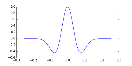
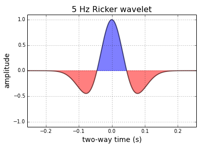
To make a wedge

We'll need a wavelet like the one we made last time. We could import it, if we've made one, but SciPy also has one so we can save ourselves the trouble. Remember to put %pylab inline at the top if using IPython notebook.

import numpy as np
from scipy.signal import ricker
import matplotlib.pyplot as plt

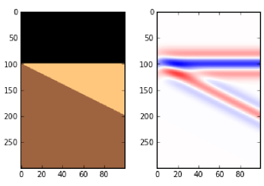
Now we need to make a physical earth model with three rock layers. In this example, let's make an acoustic impedance earth model. To keep it simple, let's define the earth model with two-way-travel time along the vertical axis (as opposed to depth). There are number of ways you could describe a wedge using math, and you could probably come up with a way that is better than mine. Here's a way:

nsamps, ntraces = [600, 500]
rock_names = ['shale 1', 'sand', 'shale 2']
rock_grid = np.zeros((n_samples, n_traces))

def make_wedge(n_samples, n_traces, layer_1_thickness, start_wedge, end_wedge):
    for j in np.arange(n_traces): 
        for i in np.arange(n_samples):      
            if i <= layer_1_thickness:      
                rock_grid[i][j] = 1    
            if i > layer_1_thickness:         
                rock_grid[i][j] = 3    
                if j >= start_wedge and i - layer_1_thickness < j-start_wedge: 
                    rock_grid[i][j] = 2
                    if j >= end_wedge and i > layer_1_thickness+(end_wedge-start_wedge):
                        rock_grid[i][j] = 3
    return rock_grid

Let's insert some numbers into our wedge function and make a particular geometry.

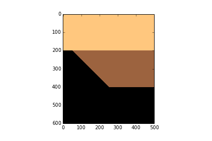
layer_1_thickness = 200
start_wedge = 50
end_wedge = 250
rock_grid = make_wedge(n_samples, n_traces, 
            layer_1_thickness, start_wedge, 
            end_wedge)

plt.imshow(rock_grid, cmap='copper_r')

Now we can give each layer in the wedge properties.

vp = np.array([3300., 3200., 3300.]) 
rho = np.array([2600., 2550., 2650.]) 
AI = vp*rho
AI = AI / 10e6 # re-scale (optional step)

Then assign values assign them accordingly to every sample in the rock model.

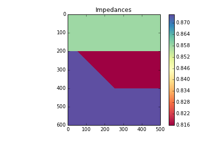
model = np.copy(rock_grid)
model[rock_grid == 1] = AI[0]
model[rock_grid == 2] = AI[1]
model[rock_grid == 3] = AI[2]

plt.imshow(model, cmap='Spectral')
plt.colorbar()
plt.title('Impedances')

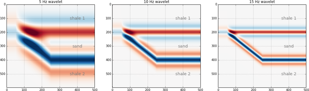
Now we can compute the reflection coefficients. I have left out a plot of the reflection coefficients, but you can check it out in the full version in the nbviewer

upper = model[:-1][:]
lower = model[1:][:]
rc = (lower - upper) / (lower + upper)
maxrc = abs(np.amax(rc))

Now we make the wavelet interact with the model using convolution. The convolution function already exists in the SciPy signal library, so we can just import it.

from scipy.signal import convolve
def make_synth(f):
    synth = np.zeros((n_samples+len(t)-2, n_traces))
    wavelet = ricker(512, 1e3/(4.*f))
    wavelet = wavelet / max(wavelet)   # normalize
    for k in range(n_traces):
        synth[:,k] = convolve(rc[:,k], wavelet)
    synth = synth[ np.ceil(len(wavelet))/2 : -np.ceil(len(wavelet))/2, : ]
    return synth

Finally, we plot the results.

frequencies = array([5, 10, 15])
plt.figure(figsize = (15, 4))
for i in np.arange(len(frequencies)):
    this_plot = make_synth(frequencies[i])
    plt.subplot(1, len(frequencies), i+1)
    plt.imshow(this_plot, cmap='RdBu', vmax=maxrc, vmin=-maxrc, aspect=1)
    plt.title( '%d Hz wavelet' % freqs[i] )
    plt.grid()
    plt.axis('tight')
    
    # Add some labels
    for i, names in enumerate(rock_names):
        plt.text(400, 100+((end_wedge-start_wedge)*i+1), names,
                 fontsize=14, color='gray',
                 horizontalalignment='center',
                 verticalalignment='center')

 

That's it. As you can see, the marriage of building mathematical functions and plotting them can be a really powerful tool you can apply to almost any physical problem you happen to find yourself working on.

You can access the full version in the nbviewer. It has a few more figures than what is shown in this post.

A day of geocomputing

I will be in Calgary in the new year and running a one-day version of this new course. To start building your own tools, pick a date and sign up:

    

To plot a wavelet

As I mentioned last time, a good starting point for geophysical computing is to write a mathematical function describing a seismic pulse. The IPython Notebook is designed to be used seamlessly with Matplotlib, which is nice because we can throw our function on graph and see if we were right. When you start your own notebook, type

ipython notebook --pylab inline

We'll make use of a few functions within NumPy, a workhorse to do the computational heavy-lifting, and Matplotlib, a plotting library.

import numpy as np
import matplotlib.pyplot as plt

Next, we can write some code that defines a function called ricker. It computes a Ricker wavelet for a range of discrete time-values t and dominant frequencies, f:

def ricker(f, length=0.512, dt=0.001):
    t = np.linspace(-length/2, (length-dt)/2, length/dt)
    y = (1.-2.*(np.pi**2)*(f**2)*(t**2))*np.exp(-(np.pi**2)*(f**2)*(t**2))
    return t, y

Here the function needs 3 input parameters; frequency, f, the length of time over which we want it to be defined, and the sample rate of the signal, dt. Calling the function returns two arrays, the time axis t, and the value of the function, y.

To create a 5 Hz Ricker wavelet, assign the value of 5 to the variable f, and pass it into the function like so,

f = 5
t, y = ricker (f)

To plot the result,

plt.plot(t, y)

But with a few more commands, we can improve the cosmetics,

plt.figure(figsize=(7,4))
plt.plot( t, y, lw=2, color='black', alpha=0.5)
plt.fill_between(t, y, 0,  y > 0.0, interpolate=False, hold=True, color='blue', alpha = 0.5)
plt.fill_between(t, y, 0, y < 0.0, interpolate=False, hold=True, color='red', alpha = 0.5)

# Axes configuration and settings (optional)
plt.title('%d Hz Ricker wavelet' %f, fontsize = 16 )
plt.xlabel( 'two-way time (s)', fontsize = 14)
plt.ylabel('amplitude', fontsize = 14)
plt.ylim((-1.1,1.1))
plt.xlim((min(t),max(t)))
plt.grid()
plt.show()

Next up, we'll make this wavelet interact with a model of the earth using some math. Let me know if you get this up and running on your own.

Let's do it

It's short notice, but I'll be in Calgary again early in the new year, and I will be running a one-day version of this new course. To start building your own tools, pick a date and sign up:

    

Coding to tell stories

Last week, I was in Calgary on family business, but I took an afternoon to host a 'private beta' for a short course that I am creating for geoscience computing. I invited about twelve familiar faces who would be provide gentle and constuctive feedback. In the end, thirteen geophysicists turned up, seven of whom I hadn't met before. So much for familiarity.

I spent about two and half hours stepping through the basics of the Python programming language, which I consider essential material — getting set up with Python via Enthought Canopy, basic syntax, and so on. In the last hour of the afternoon, I steamed through a number of geoscientific examples to showcase exercises for this would-be course. 

Here are three that went over well. Next week, I'll reveal the code for making these images. I might even have a go at converting some of my teaching materials from IPython Notebook to HTML:

To plot a wavelet

The Ricker wavelet is a simple analytic function that is used throughout seismology. This curvaceous waveform is easily described by a single variable, the dominant frequency of its many contituents frequencies. Every geophysicist and their cat should know how to plot one: 

To make a wedge

Once you can build a wavelet, the next step is to make that wavelet interact with the earth. The convolution of the wavelet with this 3-layer impedance model yields a synthetic seismogram suitable for calibrating seismic signals to subtle stratigraphic geometries. Every interpreter should know how to build a wedge, with site-specific estimates of wavelet shape and impedance contrasts. Wedge models are important in all instances of dipping and truncated layers at or below the limit of seismic resolution. So basically they are useful all of the time. 

To make a 3D viewer

The capacity of Python to create stunning graphical displays with merely a few (thoughtful) lines of code seemed to resonate with people. But make no mistake, it is not easy to wade through the hundreds of function arguments to access this power and richness. It takes practice. It appears to me that practicing and training to search for and then read documentation, is the bridge that carries people from the mundane to the empowered.

This dry-run suggested to me that there are at least two markets for training here. One is a place for showing what's possible — "Here's what we can do, now let’s go and build it". The other, more arduous path is the coaching, support, and resources to motivate students through the hard graft that follows. The former is centered on problem solving, the latter is on problem finding, where the work and creativity and sweat is. 

Would you take this course? What would you want to learn? What problem would you bring to solve?

Update on 2013-12-10 13:17 by Evan Bianco

Update: the first follow-up post in this series is a code-based tutorial on how to plot a wavelet, and has an announcement about two 1-day events I will be holding in Calgary in the new year (January 10, and January 13, 2014).

Which brittleness index?

A few weeks ago I looked at the concept — or concepts — of brittleness. There turned out to be lots of ways of looking at it. We decided to call it a rock behaviour rather than a property. And we determined to look more closely at some different ways to define it. Here they are...

Some brittleness indices

There are lots of 'definitions' of brittleness in the literature. Several of them capture the relationship between compressive and tensile strength, σ_C and σ_T respectively. This is potentially useful, because we measure uniaxial compressive strength in the standard triaxial rig tests that have become routine in shale studies... but we don't usually find the tensile strength, because it's much harder to measure. This is unfortunate, because hydraulic fracturing is initially a tensile failure (though reactivation and other failure modes do occur — see Williams-Stroud et al. 2012).

Altindag (2003) gave the following three examples of different brittleness indices. In turn, they are the strength ratio, a sort of relative strength contrast, and the mean strength (his favourite):

This is just the start, once you start digging, you'll find lots of others. Like Hucka & Das's (1974) round-up I wrote about last time, one thing they have in common is that they capture some characteristic of rock failure. That is, they do not rely on implicit rock properties.

Another point to note. Bažant & Kazemi (1990) gave a way to de-scale empirical brittleness measures to account for sample size — not surprisingly, this sort of 'real world adjustment' starts to make things quite complicated. Not so linear after all.

What not to do

The prevailing view among many interpreters is that brittleness is proportional to Young's modulus and/or Poisson's ratio, and/or a linear combination of these. We've reported a couple of times on what Lev Vernik (Marathon) thinks of the prevailing view: we need to question our assumptions about isotropy and linear strain, and computing shale brittleness from elastic properties is not physically meaningful. For one thing, you'll note that elastic moduli don't have anything to do with rock failure.

The Young–Poisson brittleness myth started with Rickman et al. 2008, SPE 115258, who presented a rather ugly representation of a linear relationship (I gather this is how petrophysicists like to write equations). You can see the tightness of the relationship for yourself in the data.

If I understand  the notation, this is the same as writing B = 7.14E – 200ν + 72.9, where E is (static) Young's modulus and ν is (static) Poisson's ratio. It's an empirical relationship, based on the data shown, and is perhaps useful in the Barnett (or wherever the data are from, we aren't told). But, as with any kind of inversion, the onus is on you to check the quality of the calibration in your rocks. 

What's left?

Here's Altindag (2003) again:

Brittleness, defined differently from author to author, is an important mechanical property of rocks, but there is no universally accepted brittleness concept or measurement method...

This leaves us free to worry less about brittleness, whatever it is, and focus on things we really care about, like organic matter content or frackability (not unrelated). The thing is to collect good data, examine it carefully with proper tools (Spotfire, Tableau, R, Python...) and find relationships you can use, and prove, in your rocks.

References

Altindag, R (2003). Correlation of specific energy with rock brittleness concepts on rock cutting. The Journal of The South African Institute of Mining and Metallurgy. April 2003, p 163ff. Available online.

Hucka V, B Das (1974). Brittleness determination of rocks by different methods. Int J Rock Mech Min Sci Geomech Abstr 10 (11), 389–92. DOI:10.1016/0148-9062(74)91109-7.

Rickman, R, M Mullen, E Petre, B Grieser, and D Kundert (2008). A practical use of shale petrophysics for stimulation design optimization: all shale plays are not clones of the Barnett Shale. SPE 115258, DOI: 10.2118/115258-MS.

Williams-Stroud, S, W Barker, and K Smith (2012). Induced hydraulic fractures or reactivated natural fractures? Modeling the response of natural fracture networks to stimulation treatments. American Rock Mechanics Association 12–667. Available online.

Great geophysicists #10: Joseph Fourier

Joseph Fourier, the great mathematician, was born on 21 March 1768 in Auxerre, France, and died in Paris on 16 May 1830, aged 62. He's the reason I didn't get to study geophysics as an undergraduate: Fourier analysis was the first thing that I ever struggled with in mathematics.

Fourier was one of 12 children of a tailor, and had lost both parents by the age of 9. After studying under Lagrange at the École Normale Supérieure, Fourier taught at the École Polytechnique. At the age of 30, he was an invited scientist on Napoleon's Egyptian campaign, along with 55,000 other men, mostly soldiers:

Citizen, the executive directory having in the present circumstances a particular need of your talents and of your zeal has just disposed of you for the sake of public service. You should prepare yourself and be ready to depart at the first order.
Herivel, J (1975). Joseph Fourier: The Man and the Physicist, Oxford Univ. Press.

He stayed in Egypt for two years, helping found the modern era of Egyptology. He must have liked the weather because his next major work, and the one that made him famous, was Théorie analytique de la chaleur (1822), on the physics of heat. The topic was incidental though, because it was really his analytical methods that changed the world. His approach of decomposing arbitrary functions into trignometric series was novel and profoundly useful, and not just for solving the heat equation. 

Fourier as a geophysicist

Late last year, Evan wrote about the reason Fourier's work is so important in geophysical signal processing in Hooray for Fourier! He showed how we can decompose time-based signals like seismic traces into their frequency components. And I touched the topic in K is for Wavenumber (decomposing space) and The spectrum of the spectrum (decomposing frequency itself, which is even weirder than it sounds). But this GIF (below) is almost all you need to see both the simplicity and the utility of the Fourier transform. 

In this example, we start with something approaching a square wave (red), and let's assume it's in the time domain. This wave can be approximated by summing the series of sine waves shown in blue. The amplitudes of the sine waves required are the Fourier 'coefficients'. Notice that we needed lots of time samples to represent this signal smoothly, but require only 6 Fourier coefficients to carry the same information. Mathematicians call this a 'sparse' representation. Sparsity is a handy property because we can do clever things with sparse signals. For example, we can compress them (the basis of the JPEG scheme), or interpolate them (as in CGG's REVIVE processing). Hooray for Fourier indeed.

The watercolour caricature of Fourier is by Julien-Leopold Boilly from his work Album de 73 Portraits-Charge Aquarelle’s des Membres de I’Institute (1820); it is in the public domain.

Read more about Fourier on his Wikipedia page — and listen to this excellent mini-biography by Marcus de Sautoy. And check out Mostafa Naghizadeh's chapter in 52 Things You Should Know About Geophysics. Download the chapter for free!

What is brittleness?

Brittleness is an important rock characteristic, but impossible to define formally because there are so many different ways of looking at it. For this reason, Tiryaki (2006) suggests we call it a rock behaviour, not a rock property.

Indeed, we're not really interested in brittleness, per se, because it's not very practical information on its own. Mining engineers are concerned with a property called cuttability — and we can think of this as conceptually analogous to the property that interests lots of geologsts, geophysicists, and engineers in petroleum, geothermal, and hydrology: frackability. In materials science, the inverse property — the ability of a rock to resist fracture — is called fracture toughness. 

What is brittleness not?

• It's not the same as frackability, or other things you might be interested in.
• It's not a simple rock property like, say, density or velocity. Those properties are condition-dependent too, but we agree on how to measure them.
• It's not proportional to any elastic moduli, or a linear combination of Young's modulus and Poisson's ratio, despite what you might have heard.

So what is it then?

It depends a bit what you care about. How the rock deforms under stress? How much energy it takes to break it? What happens when it breaks? Hucka and Das (1974) rounded up lots of ways of looking at it. Here are a few:

• Brittle rocks undergo little to no permanent deformation before failure and, depending on the test conditions, may occur suddenly and catastrophically.
• Brittle rocks undergo little or no ductile deformation past the yield point (or elastic limit) of the rock. Note that some materials, including many rocks, have no well-defined yield point because they have non-linear elasticity.
• Brittle rocks absorb relatively little energy before fracturing. The energy absorbed is equal to the area under the stress-strain curve (see figure).
• Brittle rocks have a strong tendency to fracture under stress.
• Brittle rocks break with a high ratio of fine to coarse fragments.

All of this is only made more complicated by the fact that there are lots of kinds of stress: compression, tension, shear, torsion, bending, and impact... and all of these can operate in multiple dimensions, and on multiple time scales. Suddenly a uniaxial rig doesn't quite seem like enough kit.

It will take a few posts to really get at brittleness and frackability. In future posts we'll look at relevant rock properties and how to measure them, the difference between static and dynamic measurements, and the multitude of brittleness indices. Eventually, we'll get on to what all this means for seismic waves, and ask whether frackability is something we can reasonably estimate from seismic data.

Meanwhile, if you have observations or questions to share, hit us in the comments. 

References and further reading
Hucka V, B Das (1974). Brittleness determination of rocks by different methods. Int J Rock Mech Min Sci Geomech Abstr 10 (11), 389–92. DOI:10.1016/0148-9062(74)91109-7
Tiryaki (2006). Evaluation of the indirect measures of rock brittleness and fracture toughness in rock cutting. The Journal of The South African Institute of Mining and Metallurgy 106, June 2006. Available online.

Update on 2014-06-12 01:21 by Matt Hall

Don't miss the later post, Which brittleness index?

P is for Phase

Seismic is about acoustic vibration. The archetypal oscillation, the sine wave, describes the displacement y of a point around a circle. You only need three pieces of information to describe it perfectly: the size of the circle, the speed at which it rotates around the circle, and where it starts from expressed as an angle. These quantities are better known as the amplitude, frequency, and phase respectively. These figures show how varying each of them affects the waveform:

So phase describes the starting point as an angle, but notice that this manifests itself as an apparent lateral shift in the waveform. For seismic data, this means a time shift. More on this later. 

What about seismic?

We know seismic signals are not so simple — they are not repetitive oscillations — so why do the words amplitude, frequency and phase show up so often? Aren't these words horribly inadequate?

Not exactly. Fourier's methods allow us to construct (and deconstruct) more complicated signals by adding up a series of sine waves, as long as we get the amplitude, frequency and phase values right for each one of them. The tricky part, and where much of where the confusion lies, is that even though you can place your finger on any point along a seismic trace and read off a value for amplitude, you can't do that for frequency or phase. The information for those are only unlocked through spectroscopy.

Phase shifts or time shifts?

The Ricker wavelet is popular because it can easily be written analytically, and it is comprised of a considerable number of sinusoids of varying amplitudes and frequencies. We might refer to a '20 Hz Ricker wavelet' but really it contains a range of frequencies. The blue curve shows the wavelet with phase = 0°, the purple curve shows the wavelet with a phase shift of π/3 = 60° (across all frequencies). Notice how the frequency content remains unchanged.

So for a seismic reflection event (below), phase takes on a new meaning. It expresses a time offset between the reflection and the maximum value on the waveform. When the amplitude maximum is centered at the reflecting point, it is equally shaped on either side — we call this zero phase. Notice how variations in the phase of the event alter the relative position of the peak and sidelobes. The maximum amplitude of the event at 90° is only about 80% of the amplitude at zero phase. This is why I like to plot traces along with their envelope (the grey lines). The envelope contains all possible phase rotations. Any event whose maximum value does not align with the maximum on the envelope is not zero phase.

Understanding the role of phase in time series analysis is crucial for both data processors aiming to create reliable data, and interpreters who operate under the assertion that subtle variations in waveform shape can be attributed to underlying geology. Waveform classification is a powerful attribute... but how reliable is it?

In a future post, I will cover the concept of instantaneous phase on maps and sections, and some other practical interpretation tips. If you have any of your own, share them in the comments.

Additional reading
Liner, C (2002). Phase, phase, phase. The Leading Edge 21, p 456–7. Abstract online.

Great geophysicists #9: Ernst Chladni

Ernst Chladni was born in Wittenberg, eastern Germany, on 30 November 1756, and died 3 April 1827, at the age of 70, in the Prussian city of Breslau (now Wrocław, Poland). Several of his ancestors were learned theologians, but his father was a lawyer and his mother and stepmother from lawyerly families. So young Ernst did well to break away into a sound profession, ho ho, making substantial advances in acoustic physics. 

Chladni, 'the father of acoustics', conducted a large number of experiments with sound, measuring the speed of sound in various solids, and — more adventurously — in several gases too, including oxygen, nitrogen, and carbon dioxode. Interestingly, though I can find only one reference to it, he found that the speed of sound in Pinus sylvestris was 25% faster along the grain, compared to across it — is this the first observation of acoustic anisotropy? 

The experiments Chladni is known for, however, are the plates. He effectively extended the 1D explorations of Euler and Bernoulli in rods, and d'Alembert in strings, to the 2D realm. You won't find a better introduction to Chladni patterns than this wonderful blog post by Greg Gbur. Do read it — he segués nicely into quantum mechanics and optics, firmly linking Chladni with the modern era. To see the patterns forming for yourself, here's a terrific demonstration (very loud!)...

The drawings from Chladni's book Die Akustik are almost as mesmerizing as the video. Indeed, Chladni toured most of mainland Europe, demonstrating the figures live to curious Enlightenment audiences. When I look at them, I can't help wondering if there is some application for exploration geophysics — perhaps we are missing something important in the wavefield when we sample with regular acquisition grids?

References

Chladni, E, Die Akustik, Breitkopf und Härtel, Leipzig, 1830. Amazingly, this publishing company still exists.

Read more about Chladni in Wikipedia and in monoskop.org — an amazing repository of information on the arts and sciences. 

This post is part of a not-very-regular series of posts on important contributors to geophysics. It's going rather slowly — we're still in the eighteenth century. See all of them, and do make suggestions if we're missing some!

Grand challenges, anisotropy, and diffractions

Some more highlights from the two final days of the SEG Annual Meeting in Houston.

Grand challenges

On Friday, I reported on Chevron's take on the unsolved problems in petroleum geoscience. It was largely about technology. Ken Tubman, VP of Geoscience and Reservoir Engineering at ConocoPhillips gave an equally compelling outlook on some different issue. He had five points:

• Protect the base — Fighting the decline of current production is more challenging than growing production.
• Deepwater — Recent advances in drilling are providing access to larger fields in deep water, and compressed sampling in seismic will make exploration more efficient.
• Unconventionals — In regard to the shale gas frenzy, it is not yet obvious why these reservoirs produce the way that they do. Also, since resource plays are so massive, a big challenge will be shooting larger surveys on land.
• Environment and safety — Containment assurance is more critical than pay-zone management, and geophysics will find an expanding role in preventing and diagnosing environmental and safety issues.
• People — Corporations are concerned about maintaining world class people. Which will only become more difficult as the demographic bump of senior knowledge heads off into retirement.

The Calgary crowd that harvested the list of unsolved problems at our unsession in May touched on many of these points, and identified many others that went unmentioned in this session.

Driving anisotropic ideas

In the past, seismic imaging and wave propagation were almost exclusively driven by isotropic ideas. In the final talk of the technical program, Leon Thomsen asserted that the industry has been doing AVO wrong for 30 years, and doing geomechanics wrong for 5 years. Three take-aways:

• Isotropy is no longer an acceptable approximation. It is conceptually flawed to relate Young's modulus (an elastic property), to brittleness (a mode of failure). 
• Abolish the terms vertically transverse isotropy (VTI), and horizontally transverse isotropy (HTI) from our vocabulary; how confusing to have types of anisotropy with isotropy in the name! Use polar anisotropy (for VTI), and azimuthal anisotropy (for HTI) instead.
• λ₁₃ is a simple expression of P-wave modulus M, and Thomsen's polar anisotropy parameter δ, so it should be attainable with logs.

Bill Goodway, whose work with elasticity has been criticized by Thomsen, walked to the microphone and pointed out to both the speaker and audience, that the tractability of λ₁₃ is what he has been saying all along. Colin Sayers then stood up to reiterate that geomechanics is the statistics of extremes. Anisotropic rock physics is uncontestable, but the challenge remains to find correlations with things we actually measure.

Thomas Young's sketch of 2-slit diffraction, which he showed to the Royal Society in 1803.

Imaging fractures using diffractions

Diffractions are fascinating physical phenomena that occur when the conditions of wave propagation change dramatically. They are a sort of grey zone between reflection and scattering, and can be used to resolve fractures in the subsufrace. The question is whether or not there is enough diffraction energy to detect the fractures; it can be 10× smaller than a specular reflection, so one needs very good data acquisition. Problem is, we must subtract reflections — which we deliberately optimized for — from the wavefield to get diffractions. Evgeny Landa, from Opera Geophysical, was terse, 'we must first study noise, in this case the noise is the reflections... We must study the enemy before we kill it.'

Prospecting with plate tectonics

The Santos, Campos, and Espirito Basins off the coast of Brazil contain prolific oil discoveries and, through the application of plate tectonics, explorers have been able to extend the play concepts to offshore western Africa. John Dribus, Geological Advisor at Schlumberger, described a number of discoveries as 'kissing cousins' on either side of the Atlantic, using fundamental concepts of continental margin systems and plate tectonics (read more here). He spoke passionately about big ideas, and acknowledged collaboration as a necessity: 'if we don't share our knowledge we re-invent the wheel, and we can't do that any longer'.

In the discussion session afterwards, I asked him to comment on offshore successes, which has historically hovered around 14–18%. He noted that a step change — up to about 35% — in success occured in 2009, and he gave 3 causes for it: 

• Seismic imaging around 2005 started dealing with anisotropy appropriately, getting the images right.
• Improved understanding of maturation and petroleum system elements that we didn’t have before.
• Access to places we didn’t have access to before.

Although the workshop format isn't all that different from the relentless PowerPoint of the technical talks, it did have an entirely different feeling. Was it the ample discussion time, or the fact that the trade show, now packed neatly in plywood boxes, boosted the signal:noise? Did you see anything remarkable at a workshop last week? 

Key technology trends in earth science

Yesterday, I went to the workshop entitled, Grand challenges and research opportunities in geophysics, organized by Cengiz Esmersoy, Wafik Beydoun, Colin Sayers, and Yoram Shoham. I was curious if there'd be overlap with the Unsolved Problems Unsession we hosted in Calgary, and had reservations about it being an overly fluffy talkshop, but it was much better than I expected.

Ken Tubman, VP of Geosciences and Reservoir Engineering at ConocoPhillips, gave a splendid talk to open the session. But it was the third talk of the session, from Mark Koelmel, General Manager of Earth Sciences at Chevron, that resonated most with me. He highlighted 5 trends in applied earth science.

Data and information management

Data volumes are expanding with Moore's law. Chevron has more than 15 petabytes of data, by 2020 they will have more than 100PB. Koelmel postulated that spatial metadata and tagging will become pervasive and our data formats will have to evolve accordingly. Instead of managing ridiculously large amounts of data, a better solution may be to 'tag it and chuck it in the closet' — Google's approach to the web (and we know the company has been exploring the use of Hadoop). Beyond hardware, he stressed that new industry standards are needed now. The status quo is holding us back.

Full azimuth seismic data

Only recently have we been able to wield the computing power to deal with the kind of processes needed for full-waveform inversion. It's not only because of data volumes that new processing facilities will not be cheap — or small. He predicted processing centres that resemble small cities in terms of their power consumption. An interesting notion of energy for energy, and the reason for recent massive growth in Google's power production capability. (Renewables for power, oil for cooling... how funny would that be?)

Interpretive seismic processing and imaging

Interpretation, and processing are actually the same thing. The segmentation of seismic technology will have to be stitched back together. Imagine the interpreter working on field data, with a mixing board to produce just the right image for today's work. How will service companies (who acquire data and make images), and operators (who interpret data and make prospects) merge their efforts? We may have to consider different business relationships.

Full-cycle interpretation systems

The current state of integration is sequential at best, each node in a workflow produces static inputs for the next step, with minimal iteration in between. Each component of the sequence typically ends with 'throwing things over the wall' to the next node. With this process, the uncertainties are cumulative throughout, which is unnerving because we don't often know what the uncertainties are. Koelmel's desired future state is one of seamless geophysical processing, static model-building, and dynamic reservoir simulation. It won't reduce uncertainties altogether, but by design it will make them easier to identify and addressed.

Intellectual property

The number of patents filed in this industry has more than tripled in the last decade. I assumed Koelmel was going to give a Big Oil lecture on secrecy and patents, touting them as a competitive advantage. He said just the opposite. He asserted that industries with excessive patenting (think technology, and Big Pharma) make innovation difficult. Chevron is no stranger to the patent processes, filing 125 patents both in 2012 and in 2011, but this is peanuts compared to Schlumberger (462 in 2012) and IBM (6457 in 2012). 

The challenges geophysicists are facing are not our own. They stem from the biggest problems in the industry, which are of incredible importance to mankind. Perhaps expanding the value proposition to such heights is more essential than ever. Geophysics matters.