Joseph Fourier, the great mathematician, was born on 21 March 1768 in Auxerre, France, and died in Paris on 16 May 1830, aged 62. He's the reason I didn't get to study geophysics as an undergraduate: Fourier analysis was the first thing that I ever struggled with in mathematics.

Fourier was one of 12 children of a tailor, and had lost both parents by the age of 9. After studying under Lagrange at the École Normale Supérieure, Fourier taught at the École Polytechnique. At the age of 30, he was an invited scientist on Napoleon's Egyptian campaign, along with 55,000 other men, mostly soldiers:

Citizen, the executive directory having in the present circumstances a particular need of your talents and of your zeal has just disposed of you for the sake of public service. You should prepare yourself and be ready to depart at the first order.
Herivel, J (1975). Joseph Fourier: The Man and the Physicist, Oxford Univ. Press.

He stayed in Egypt for two years, helping found the modern era of Egyptology. He must have liked the weather because his next major work, and the one that made him famous, was Théorie analytique de la chaleur (1822), on the physics of heat. The topic was incidental though, because it was really his analytical methods that changed the world. His approach of decomposing arbitrary functions into trignometric series was novel and profoundly useful, and not just for solving the heat equation.

Fourier as a geophysicist

Late last year, Evan wrote about the reason Fourier's work is so important in geophysical signal processing in Hooray for Fourier! He showed how we can decompose time-based signals like seismic traces into their frequency components. And I touched the topic in K is for Wavenumber (decomposing space) and The spectrum of the spectrum (decomposing frequency itself, which is even weirder than it sounds). But this GIF (below) is almost all you need to see both the simplicity and the utility of the Fourier transform.

In this example, we start with something approaching a square wave (red), and let's assume it's in the time domain. This wave can be approximated by summing the series of sine waves shown in blue. The amplitudes of the sine waves required are the Fourier 'coefficients'. Notice that we needed lots of time samples to represent this signal smoothly, but require only 6 Fourier coefficients to carry the same information. Mathematicians call this a 'sparse' representation. Sparsity is a handy property because we can do clever things with sparse signals. For example, we can compress them (the basis of the JPEG scheme), or interpolate them (as in CGG's REVIVE processing). Hooray for Fourier indeed.

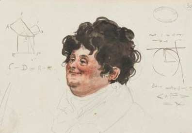
The watercolour caricature of Fourier is by Julien-Leopold Boilly from his work Album de 73 Portraits-Charge Aquarelle’s des Membres de I’Institute (1820); it is in the public domain.