
Fabric textures
/Beyond the traditional, well-studied attributes that I referred to last time, are a large family of metrics from image processing and robot vision. The idea is to imitate the simple pattern recognition rules our brains intuitively and continuously apply when we look at seismic data: how do the data look? How smooth or irregular are the reflections? If you thought the adjectives I used for my tea towels were ambiguous, I assure you seismic will be much more cryptic.
In three-dimensional data, texture is harder to see, difficult to draw, and impossible to put on a map. So when language fails us, discard words altogether and use numbers instead. While some attributes describe the data at a particular place (as we might describe a photographic pixel as 'red', 'bright', 'saturated'), other attributes describe the character of the data in a small region or kernel ('speckled', 'stripy', 'blurry').
Texture by numbers
I converted the colour image from the previous post to a greyscale image with 256 levels (a bit-depth of 8) to match this notion of scalar seismic data samples in space. The geek speak is that I am computing local grey-level co-occurence matrices (or GLCMs) in a moving window around the image, and then evaluating some statistics of the local GLCM for each point in the image. These statistics are commonly called Haralick textures. Choosing the best kernel size will depend on the scale of the patterns. The Haralick textures are not particularly illustrative when viewed on their own but they can be used for data clustering and classification, which will be the topic of my next post.
- Step 1: Reduce the image to 256 grey-levels
- Step 2: For every pixel, compute a co-occurrence matrix from a p by q kernel (p, q = 15 for my tea towel photo)
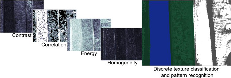
- Step 3: For every pixel, compute the Haralick textures (Contrast, Correlation, Energy, Homogeneity) from the GLCM
Textures in seismic data
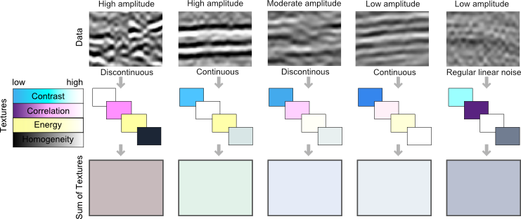
Here are a few tiles of seismic textures that I have loosely labeled as "high-amplitude continous", "high-amplitude discontinuous", "low-amplitude continuous", etc. You certainly might choose different words to describe them, but each has a unique and objective set of Haralick textures. I have explicitly represented the value of each's texture as a color; using cyan for contrast, magenta for correlation, yellow for energy, and black for homogeneity. Thus, the four Haralick textures span the CMYK color space. Merging these components back together into a single color gives you a sense of the degree of difference across the tiles. For instance, the high-amplitude continuous tile, is characterized by high contrast and high energy, but low correlation, relative to the low-amplitude continuous tile. Their textures are similar, so obviously, they map to similar color values in CMYK color space. Whether or not they are truly discernable is the challenge we offer to data clustering; be it employed by visual inspection or computational force.
Further reading:
Gao, D., 2003, Volume texture extraction for 3D seismic visualization and interpretation, Geophysics, 64, No. 4, 1294-1302
Haralick, R., Shanmugam, K., and Dinstein, I., 1973, Textural features for image classification: IEEE Tran. Systems, Man, and Cybernetics, SMC-3, 610-621.
Mryka Hall-Beyer has a great tutorial at http://www.fp.ucalgary.ca/mhallbey/tutorial.htm for learning more about GLCMs.
Images in this post were made using MATLAB, FIJI and Inkscape.


 Except where noted, this content is licensed