x lines of Python: contour maps

Difficulty rating: EASY

Following on from the post a couple of weeks ago about colourmaps, I wanted to poke into contour maps a little more. Ostensibly, making a contour plot in matplotlib is a one-liner:

plt.contour(data)

But making a contour plot look nice takes a little more work than most of matplotlib's other plotting functions. For example, to change the contour levels you need to make an array containing the levels you want... another line of code. Adding index contours needs another line. And then there's all the other plotty stuff.

Here's what we'll do:

  1. Load the data from a binary NumPy file.
  2. Check the data looks OK.
  3. Get the min and max values from the map.
  4. Generate the contour levels.
  5. Make a filled contour map and overlay contour lines.
  6. Make a map with index contours and contour labels.

The accompanying notebook sets out all the code you will need. You can even run the code right in your browser, no installation required.

Here's the guts of the notebook:

 
import numpy as np
import matplotlib.pyplot as plt

seabed = np.load('../data/Penobscot_Seabed.npy')
seabed *= -1
mi, ma = np.floor(np.nanmin(seabed)), np.ceil(np.nanmax(seabed))
step = 2
levels = np.arange(10*(mi//10), ma+step, step)
lws = [0.5 if level % 10 else 1 for level in levels]

# Make the plot
fig = plt.figure(figsize=(12, 8))
ax = fig.add_subplot(1,1,1)
im = ax.imshow(seabed, cmap='GnBu_r', aspect=0.5, origin='lower')
cb = plt.colorbar(im, label="TWT [ms]")
cb.set_clim(mi, ma)
params = dict(linestyles='solid', colors=['black'], alpha=0.4)
cs = ax.contour(seabed, levels=levels, linewidths=lws, **params)
ax.clabel(cs, fmt='%d')
plt.show()

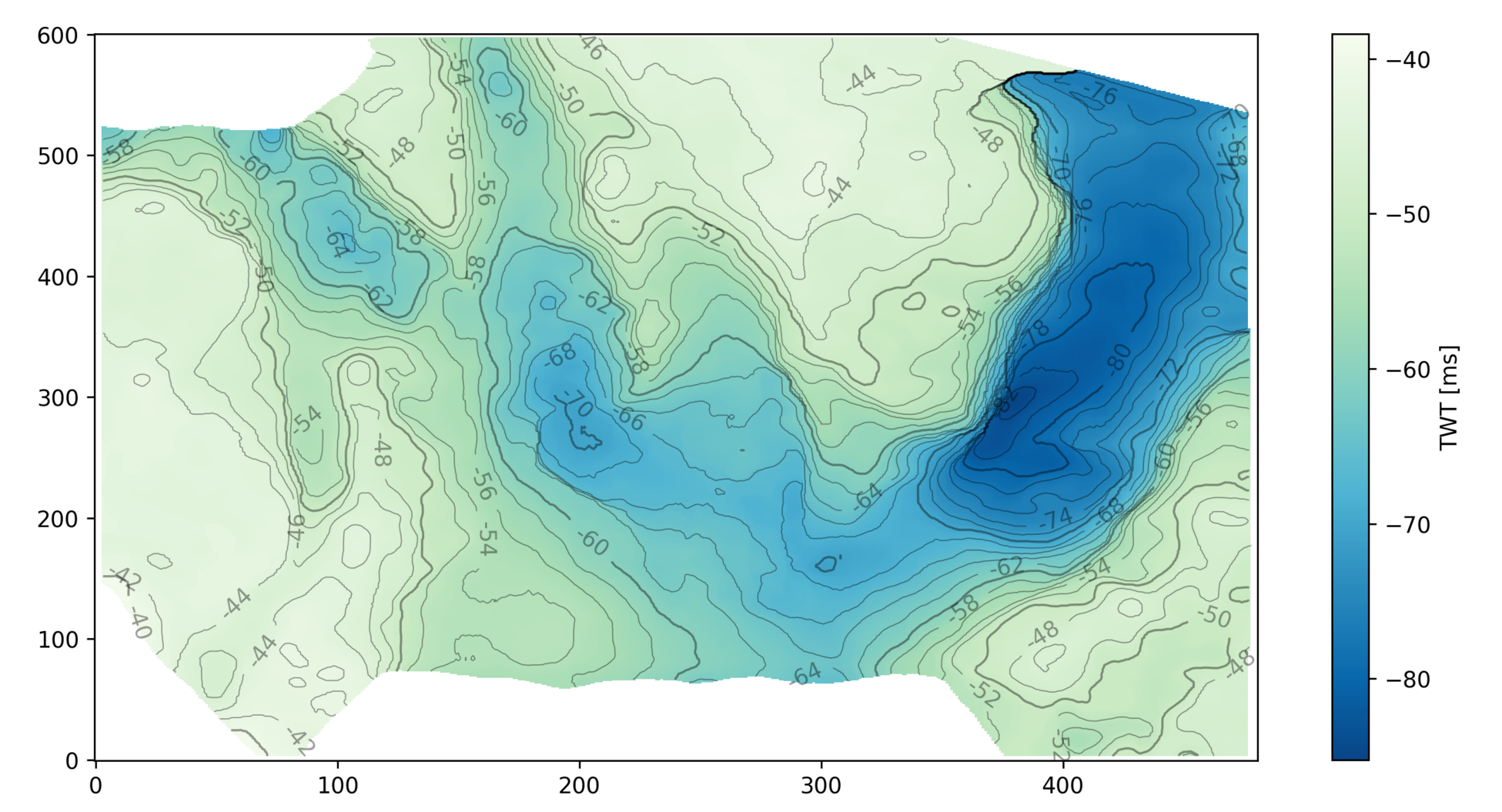
This produces the following plot:

my_map.png

Old skool plot tool

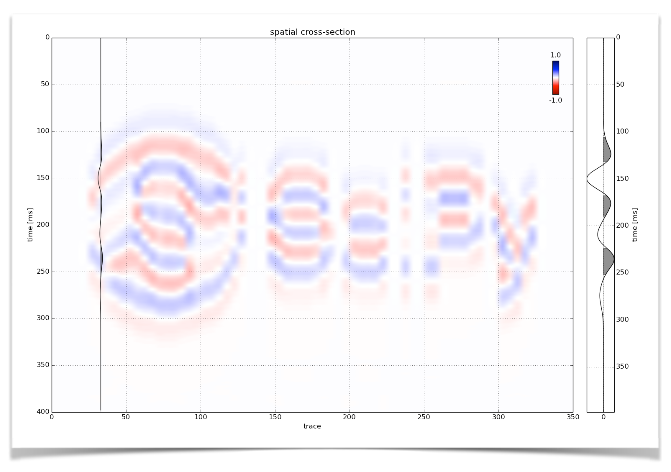
It's not very glamorous, but sometimes you just want to plot a SEG-Y file. That's why we crafted seisplot. OK, that's why we cobbled seisplot together out of various scripts and functions we had lying around, after a couple of years of blog posts and Leading Edge tutorials and the like.

Pupils of the old skool — when everyone knew how to write a bash script, pencil crayons and lead-filled beanbags ruled the desktop, and Carpal Tunnel Syndrome was just the opening act to the Beastie Boys — will enjoy seisplot. For a start, it's command line only: 

    python seisplot.py -R -c config.py ~/segy_files -o ~/plots

Isn't that... reassuring? In this age of iOS and Android and Oculus Rift... there's still the command line interface.

Features galore

So what sort of features can you look forward to? Other than all the usual things you've come to expect of subsurface software, like a complete lack of support or documentation. (LOL, I'm kidding.) Only these awesome selling points:

  • Make wiggle traces or variable density plots... or don't choose — do both!
  • If you want, the script will descend into subdirectories and make plots for every SEG-Y file it finds.
  • There are plenty of colourmaps to choose from, or if you're insane you can make your own.
  • You can make PNGs, JPGs, SVGs or PDFs. But not CGM, sorry about that.

Well, I say 'selling points', but the tool is 100% free. We think this is a fair price. It's also open source of course, so please — seriously, please — improve the source code, then share it with the world! The code is in GitHub, natch.

Never go full throwback

There is one more feature: you can go full throwback and add scribbles and coffee stains. Here's one for your wall:


The 2D seismic line in this post is from the USGS NPRA Seismic Data Archive, and are in the public domain. This is line number 31-81-PR (links directly to SEG-Y file).

Monday highlights from SEG

Ben and I are in New Orleans at the 2015 SEG Annual Meeting, a fittingly subdued affair, given the industry turmoil recently. Lots of people are looking for work, others are thankful to have it.

We ran our annual Geophysics Hackathon over the weekend; I'll write more about that later this week. In a nutshell: despite a low-ish turnout, we had 6 great projects, all of them quite different from anything we've seen before. Once again, Colorado School of Mines dominated.

Beautiful maps

One of the most effective ways to make a tight scientific argument is to imagine trying to convince the most skeptical person you know that your method works. When it comes to seismic attribute analysis, I am that skeptical person.

Some of the nicest images I saw today were in the 'Attributes for Stratigraphic Analysis' session, chaired by Rupert Cole and Yuefeng Sun. For example, Tao Zhao, one of Kurt Marfurt's students, showed some beautiful images from the Waka 3D offshore New Zealand (Zhao & Marfurt). He used 2D colourmaps to co-render two attributes together, along with semblance mapped to opacity on a black layer, and were very nice to look at. However I was left wondering, and not for the first time, how we can do a better job calibrating those maps to geology. We (the interpretation community) need to stop side-stepping that issue; it's central to our credibility. Even if you have no wells, as in this study, you can still use forward models, analogs, or at least interpretation by a sedimentologist, preferably two.

© SEG and Zhao & Marfurt. Left to right: Peak spectral frequency and peak spectral magnitude; GLCM homogeneity; shape index and curvedness. All of the attributes are also corendered with Sobel edge detection.

© SEG and Zhao & Marfurt. Left to right: Peak spectral frequency and peak spectral magnitude; GLCM homogeneity; shape index and curvedness. All of the attributes are also corendered with Sobel edge detection.

Pavel Jilinski at GeoTeric gave a nice talk (Calazans Muniz et al.) about applying some of these sort of fancy displays to a large 3D dataset in Brazil, in a collaboration with Petrobras. The RGB displays of spectral attributes were as expected, but I had not seen their cyan-magenta-yellow (CMY) discontinuity displays before. They map dip to the yellow channel, similarity to the magenta channel, and 'tensor discontinuity' to the cyan channel. No, I don't know what that means either, but the displays were pretty cool.

Publications news

This evening we enjoyed the Editor's Dinner (I coordinate a TLE column and review for Geophysics and Interpretation, so it's totally legit). Good things are coming to the publication world: adopted Canadian Mauricio Sacchi is now Editor-in-Chief, there are no more page charges for colour in Geophysics (up to 10 pages), and watch out for video abstracts next year. Also, Chris Liner mentioned that Interpretation gets 18% of its submissions from oil companies, compared to only 5% for Geophysics. And I heard, but haven't verified, that downturns result in more papers. So at least our journals are healthy. (You do read them, right?)

That's it for today (well, yesterday). More tomorrow!


References

Calazans Muniz, Moises, Thomas Proença, and Pavel Jilinski (2015). Use of Color Blend of seismic attributes in the Exploration and Production Development - Risk Reduction. SEG Technical Program Expanded Abstracts 2015: pp. 1638-1642. doi: 10.1190/segam2015-5916038.1

Zhao, Tao, and Kurt J. Marfurt (2015). Attribute assisted seismic facies classification on a turbidite system in Canterbury Basin, offshore New Zealand. SEG Technical Program Expanded Abstracts 2015: pp. 1623-1627. doi: 10.1190/segam2015-5925849.1

Corendering more attributes

My recent post on multi-attribute data visualization painted two seismic attributes from on a timeslice. Let's look now at corendering attributes extracted on a seismic horizon. I'll reproduce the example Matt gave in his post on colouring maps.

Although colour choices come down to personal preference, there are some points to keep in mind:

  • Data that varies relatively gradually across the canvas — e.g. elevation here — should use a colour scale that varies monotonically in hue and luminance, e.g. CubeHelix or Matteo Niccoli's colourmaps.
  • Data that varies relatively quickly across the canvas — e.g. my similarity data, (a member of the family that includes coherencesemblance, and so on) — should use a monochromatic colour scale, e.g. black–white. 
  • If we've chosen our colourmaps wisely, there should be some unused hues for rendering other additional attributes. In this case, there are no red hues in the elevation colourmap, so we can map redness to instantaneous amplitude.

Adding a light source

Without wanting to get too gimmicky, we can sometimes enliven the appearance of an attribute, accentuating its texture, by simulating a bumpy surface and shining a virtual light onto it. This isn't the same as casting a light source on the composite display. We can make our light source act on only one of our attributes and leave the others unchanged. 

Similarity attribute Displayed using a Greyscale Colourbar (left). Bump mapping of similarity attribute using a lightsource positioned at azimuth 350 degrees, inclination 20 degrees. 

The technique is called hill-shading. The terrain doesn't have to be a physical surface; it can be a slice. And unlike physical bumps, we're not actually making a new surface with relief, we are merely modifying the surface's luminance from an artificial light source. The result is a more pronounced texture.

One view, two dimensions, three attributes

Constructing this display takes a bit of trial an error. It wasn't immediately clear where to position the light source to get the most pronounced view. Furthermore, the amplitude extraction looked quite noisy, so I softened it a little bit using a Gaussian filter. Plus, I wanted to show only the brightest of the bright spots, so that all took a bit of fiddling.

Even though 3D data visualization is relatively common, my assertion is that it is much harder to get 3D visualization right, than for 2D. Looking at the 3 colour-bars that I've placed in the legend. I'm reminded of this difficulty of adding a third dimension; it's much harder to produce a colour-cube in the legend than a series of colour-bars. Maybe the best we can achieve is a colour-square like last time, with a colour-bar for the overlay on the side.

Check out the IPython notebook for the code used to create these figures.

The (bad) stuff of legend

What is a legend? Merriam–Webster says:

  1. A story from the past that is believed by many people but cannot be proved to be true.
  2. An explanatory list of the symbols on a map or chart.

I think we can combine these:

An explanatory list from the past that is believed by many to be useful but which cannot be proved to be.

Maybe that goes too far, sometimes you need a legend. But often, very often, you don't. At the very least, you should always try hard to make the legend irrelevant. Why, and how, can you do this? 

A case study

On the right is a non-scientific caricature of a figure from a paper I just finished reviewing for Geophysics. I won't give any more details because I don't want to pick on it unduly — lots of authors make the same mistakes.

Here are some of the things I think are confusing about this figure, detracting from the science in the paper. 

  • Making the reader cross-reference the line decoration with the legend makes it harder to make the comparison you're asking them to make. Just label the lines directly. 
  • Using unhelpful, generic names like 1, 2, and 3 for the models leads the reader into cross-reference Inception. The models were shown and explained on the previous page. 
  • Inception again: the models 1, 2, and 3 were shown in the previous figure parts (a), (b), and (c) respectively. So I had to cross-reference deeper still to really find out about them. 
  • The paper used colour elsewhere, so the use of black and white line decoration here seems unnecessary. There are other ways to ensure clarity if the paper is photocopied.
  • Everything on the same visual plane, so to speak, so the chart cannot take any more detail, such as gridlines. 

Getting better

I have tried to fix some of this in the version of the figure shown here. It's the same size as the original. The legend, such as it is, is now a visual key to the models. Careful juxtaposition of figures could obviate the need even for this extra key. The idea would be to use the colours and names of the models in every figure, to link them more intuitively.

The principles at work:

  • Reduce the fatigue of reading by labeling things directly.
  • Avoid using 'a' and 'b' or other generic names. Call the parts before and after, or 8 ms gate and 16 ms gate
  • Put things you want people to compare next to each other: models with data, output with input, etc. 
  • Use less ink for decoration, more ink for data. Gently direct the reader's attention. 

I'm sure there are other improvements we could make. Do you have any tips to share for making better figures? Leave them in the comments. 


Update, 30 Jan 2015

Some great comments came in today, and the point about black and white is well taken. Indeed, our 52 Things books are all black and white, and I end up transforming most images and figures to (I hope) make them clearer without colour. Here's how I'd do this figure in black and white.

Why don't people use viz rooms?

Matteo Niccoli asked me why I thought the use of immersive viz rooms had declined. Certainly, most big companies were building them in about 1998 to 2002, but it's rare to see them today. My stock answer was always "Linux workstations", but of course there's more to it than that.

What exactly is a viz room?

I am not talking about 'collaboration rooms', which are really just meeting rooms with a workstation and a video conference phone, a lot of wires, and wireless mice with low batteries. These were one of the collaboration technologies that replaced viz rooms, and they seem to be ubiquitous (and also under-used).

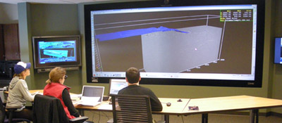
The Viz Lab at Wisconsin–Madison. Thanks to Harold Tobin for permission.A 'viz room', for our purposes here, is a dark room with a large screen, at least 3 m wide, probably projected from behind. There's a Crestron controller with greasy fingerprints on it. There's a week-old coffee cup because not even the cleaners go in there anymore. There's probably a weird-looking 3D mouse and some clunky stereo glasses. There might be some dusty haptic equipment that would work if you still had an SGI.

Why did people stop using them?

OK, let's be honest... why didn't most people use them in the first place?

  1. The rise of the inexpensive Linux workstation. The Sun UltraSPARC workstations of the late 1990s couldn't render 3D graphics quickly enough for spinning views or volume-rendered displays, so viz rooms were needed for volume interpretation and well-planning. But fast machines with up to 16GB of RAM and high-end nVidia or AMD graphics cards came along in about 2002. A full dual-headed set-up cost 'only' about $20k, compared to about 50 times that for an SGI with similar capabilities (for practical purposes). By about 2005, everyone had power and pixels on the desktop, so why bother with a viz room?
  2. People never liked the active stereo glasses. They were certainly clunky and ugly, and some people complained of headaches. It took some skill to drive the software, and to avoid nauseating spinning around, so the experience was generally poor. But the real problem was that nobody cared much for the immersive experience, preferring the illusion of 3D that comes from motion. You can interactively spin a view on a fast Linux PC, and this provides just enough immersion for most purposes. (As soon as the motion stops, the illusion is lost, and this is why 3D views are so poor for print reproduction.)
  3. They were expensive. Early adoption was throttled by expense  (as with most new technology). The room renovation might cost $250k, the SGI Onyx double that, and the projectors were $100k each. But  even if the capex was affordable, everyone forgot to include operating costs — all this gear was hard to maintain. The pre-DLP cathode-ray-tube projectors needed daily calibration, and even DLP bulbs cost thousands. All this came at a time when companies were letting techs go and curtailing IT functions, so lots of people had a bad experience with machines crashing, or equipment failing.
  4. Intimidation and inconvenience. The rooms, and the volume interpretation workflow generally, had an aura of 'advanced'. People tended to think their project wasn't 'worth' the viz room. It didn't help that lots of companies made the rooms almost completely inaccessible, with a locked door and onerous booking system, perhaps with a gatekeeper admin deciding who got to use it.
  5. Our culture of PowerPoint. Most of the 'collaboration' action these rooms saw was PowerPoint, because presenting with live data in interpretation tools is a scary prospect and takes practice.
  6. Volume interpretation is hard and mostly a solitary activity. When it comes down to it, most interpreters want to interpret on their own, so you might as well be at your desk. But you can interpret on your own in a viz room too. I remember Richard Beare, then at Landmark, sitting in the viz room at Statoil, music blaring, EarthCube buzzing. I carried on this tradition when I was at Landmark as I prepared demos for people, and spent many happy hours at ConocoPhillips interpreting 3D seismic on the largest display in Canada.  

What are viz rooms good for?

Don't get me wrong. Viz rooms are awesome. I think they are indispensable for some workflows: 

  • Well planning. If you haven't experienced planning wells with geoscientists, drillers, and reservoir engineers, all looking at an integrated subsurface dataset, you've been missing out. It's always worth the effort, and I'm convinced these sessions will always plan a better well than passing plans around by email. 
  • Team brainstorming. Cracking open a new 3D with your colleagues, reviewing a well program, or planning the next year's research projects, are great ways to spend a day in a viz room. The broader the audience, as long as it's no more than about a dozen people, the better. 
  • Presentations. Despite my dislike of PowerPoint, I admit that viz rooms are awesome for presentations. You will blow people away with a bit of live data. My top tip: make PowerPoint slides with an aspect ratio to fit the entire screen: even PowerPoint haters will enjoy 10-metre-wide slides.

What do you think? Are there still viz rooms where you work? Are there 'collaboration rooms'? Do people use them? Do you?

July linkfest

It's linkfest time again. All the links, in one handy post.

First up — I've seen some remarkable scientific visualizations recently. For example, giant ocean vortices spiralling across the globe (shame about the rainbow colourbar though). Or the trillion-particle Dark Sky Simulation images we saw at SciPy. Or this wonderful (real, not simulated) video by the Perron Group at MIT:

Staying with visuals, I highly recommend reading anything by Mike Bostock, especially if you're into web technology. The inventor of D3.js, a popular data viz library, here's his exploration of algorithms, from sampling to sorting. It's more conceptual than straight up visualization of data, but no less insightful. 

And I recently read about some visual goodness combined with one of my favourite subjects, openness. Peter Falkingham, a palaeontologist at the Royal Vetinary College and Brown University, has made a collection of 3D photographs of modern tracks and traces available to the world. He knows his data is more impactful when others can use it too.

Derald Smith and sedimentology

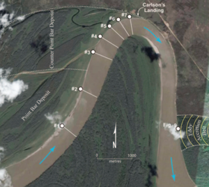
From Smith et al. (2009) in SEPM Special Publication No. 97.The geological world was darkened by the death of Derald Smith on 18 June. I met Derald a few times in connection with working on the McMurray Formation of Alberta, Canada during my time at ConocoPhillips. We spent an afternoon examining core and seismic data, and speculating about counter-point-bars, a specialty of his. He was an intuitive sedimentologist whose contributions will be remembered for many years.

Another geological Smith is being celebrated in September at the Geological Society of London's annual William Smith Meeting. The topic this year is The Future of Sequence Stratigraphy: Evolution or Revolution? Honestly, my first thought was "hasn't that conversation been going on since 1994?", but on closer inspection, it promises to be an interesting two days on 'source-to-sink', 'landscape into rock', and some other recent ideas.

The issue of patents reared up in June when Elon Musk of Tesla Motors announced the relaxation of their patents — essentially a promise not to sue anyone using one of their patented technology. He realizes that a world where lots of companies make electric vehicles is better for Tesla. I wrote a piece about patents in our industry.

Technology roundup

A few things that caught our eye online:

Last thing: did you know that the unit of acoustic impedance is the Rayl? Me neither. 


Previous linkfests: AprilJanuaryOctober.

The figure is from Smith et al. (2009), Stratigraphy of counter-point-bar and eddy accretion deposits in low-energy meander belts of the Peace–Athabasca delta, northeast Alberta, Canada. In: SEPM Special Publication No. 97, ISBN 978-1-56576-305-0, p. 143–152. It is copyright of SEPM, and used here in accordance with their terms.

Graphics that repay careful study

The Visual Display of Quantitative Information by Edward Tufte (2nd ed., Graphics Press, 2001) celebrates communication through data graphics. The book provides a vocabulary and practical theory for data graphics, and Tufte pulls no punches — he suggests why some graphics are better than others, and even condemns failed ones as lost opportunities. The book outlines empirical measures of graphical performance, and describes the pursuit of graphic-making as one of sequential improvement through revision and editing. I see this book as a sort of moral authority on visualization, and as the reference book for developing graphical taste.

Through design, the graphic artist allows the viewer to enter into a transaction with the data. High performance graphics, according to Tufte, 'repay careful study'. They support discovery, probing questions, and a deeper narrative. These kinds of graphics take a lot of work, but they do a lot of work in return. In later books Tufte writes, 'To clarify, add detail.'

A stochastic AVO crossplot

Consider this graphic from the stochastic AVO modeling section of modelr. Its elements are constructed with code, and since it is a program, it is completely reproducible.

Let's dissect some of the conceptual high points. This graphic shows all the data simultaneously across 3 domains, one in each panel. The data points are sampled from probability density estimates of the physical model. It is a large dataset from many calculations of angle-dependent reflectivity at an interface. The data is revealed with a semi-transparent overlay, so that areas of certainty are visually opaque, and areas of uncertainty are harder to see.

At the same time, you can still see every data point that makes the graphic giving a broad overview (the range and additive intensity of the lines and points) as well as the finer structure. We place the two modeled dimensions with templates in the background, alongside the physical model histograms. We can see, for instance, how likely we are to see a phase reversal, or a Class 3 response subject to the physical probability estimates. The statistical and site-specific nature of subsurface modeling is represented in spirit. All the data has context, and all the data has uncertainty.

Rules for graphics that work

Tufte summarizes that excellent data graphics should:

  • Show all the data.
  • Provoke the viewer into thinking about meaning.
  • Avoid distorting what the data have to say.
  • Present many numbers in a small space.
  • Make large data sets coherent.
  • Encourage the eye to compare different pieces of the data.
  • Reveal the data at several levels of detail, from a broad overview to the fine structure.
  • Serve a reasonably clear purpose: description, exploration, tabulation, or decoration.
  • Be closely integrated with the statistical and verbal descriptions of a data set.

The data density, or data-to-ink ratio, looks reasonably high in my crossplot, but it could like still be optimized. What would you remove? What would you add? What elements need revision?

Geophysics at SciPy 2014

Wednesday was geophysics day at SciPy 2014, the conference for scientific Python in Austin. We had a mini-symposium in the afternoon, with 4 talks and 2 lightning talks about posters.

All the talks

Here's what went on in the session...

The talks should all be online eventually. For now, you can watch my talk and Joe's (awesome) talk right here...

And also...

There have been so many other highlights at this amazing conference that I can't resist sharing a couple of the non-geophysical gems...

Last thing... If you use the scientific Python stack in your work, please consider giving as generously as you can to the NumFOCUS Foundation. Support open source!

Ternary diagrams

I like spectrums (or spectra, if you must). It's not just because I like signals and Fourier transforms, or because I think frequency content is the most under-appreciated attribute of seismic data. They're also an important thinking tool. They represent a continuum between two end-member states, both rare or unlikely; in between there are shades of ambiguity, and this is usually where nature lives.

Take the sport–game continuum. Sports are pure competition — a test of strength and endurance, with few rules and unequivocal outcomes. Surely marathon running is pure sport. Contrast that with a pure game, like darts: no fitness, pure technique. (Establishing where various pastimes lie on this continuum is a good way to start an argument in a pub.)

There's a science purity continuum too, with mathematics at one end and social sciences somewhere near the other. I wonder where geology and geophysics lie...

Degrees of freedom 

The thing about a spectrum is that it's two-dimensional, like a scatter plot, but it has only one degree of freedom, so we can map it onto one dimension: a line.

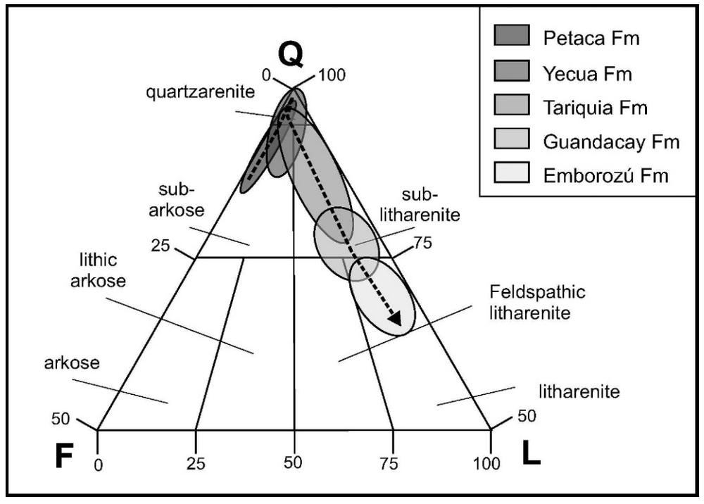
The three-dimensional equivalent of the spectrum is the ternary diagram: 3-parameter space mapped onto 2D. Not a projection, like a 3D scatter plot, because there are only two degrees of freedom — the parameters of a ternary diagram cannot be independent. This works well for volume fractions, which must sum to one. Hence their popularity for the results of point-count data, like this Folk classification from Hulk & Heubeck (2010).

We can go a step further, natch. You can always go a step further. How about four parameters with three degrees of freedom mapped onto a tetrahedron? Fun to make, not so fun to look at. But not as bad as a pentachoron.

How to make one

The only tools I've used on the battlefield, so to speak are Trinity, for ternary plots, and TetLab, for tetrahedrons (yes, I went there), both Mac OS X only, and both from Peter Appel of Christian-Albrechts-Universität zu Kiel. But there are more...

Do you use ternary plots, or are they nothing more than a cute way to show some boring data? How do you make them? Care to share any? 

The cartoon is from xkcd.com, licensed CC-BY-NC. The example diagram and example data are from Hulka, C and C Heubeck (2010). Composition and provenance history of Late Cenozoic sediments in southeastern Bolivia: Implications for Chaco foreland basin evolution and Andean uplift. Journal of Sedimentary Research 80, 288–299. DOI: 10.2110/jsr.2010.029 and available online from the authors.