A revolution in seismic acquisition?

We're in warm, sunny Calgary for the GeoConvention 2013. The conference feels like it's really embracing geophysics this year — in the past it's always felt more geological somehow. Even the exhibition floor felt dominated by geophysics. Someone we spoke to speculated that companies were holding their geological cards close to their chests, but the service companies are still happy to talk about (ahem, promote) their geophysical advances.

Are you at the conference? What do you think? Let us know in the comments.

We caught about 15 talks of the 100 or so on offer today. A few of them ignited the old whines about half-cocked proofs of efficacy. Why is it still acceptable to say that a particular seismic volume or inversion result is 'higher resolution' or 'more geological' with nothing more than a couple of sections or timeslices as evidence?

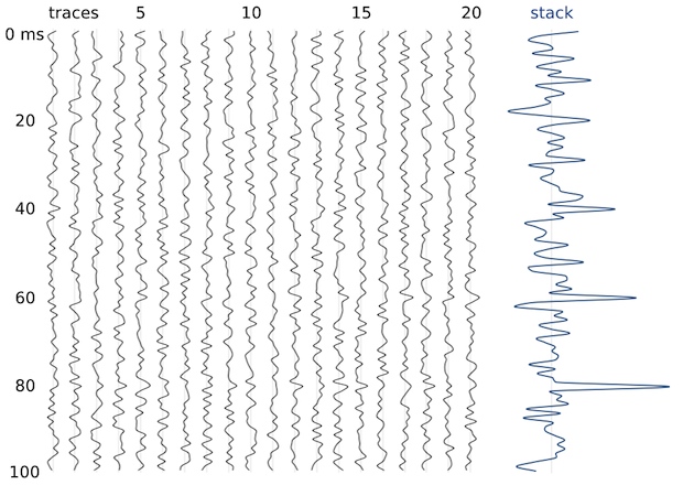
People are excited about designing seismic acquisition expressly for wavefield reconstruction. In a whole session devoted to the subject, for example, Mauricio Sacchi showed how randomization helps with regularization in processing, allowing us to either get better image quality, or to lower cost. It feels like the start of a new wave of innovation in acquisition, which has more than its fair share of recent innovation: multi-component, wide azimuth, dual-sensor, simultaneous source...

Is it a revolution? Or just the fallacy of new things looking revolutionary... until the next new thing? It's intriguing to the non-specialist. People are talking about 'beyond Nyquist' again, but this time without inducing howls of derision. We just spent an hour talking about it, and we think there's something deep going on... we're just not sure how to articulate it yet.

Unsolved problems

We were at the conference today, but really we are focused on the session we're hosting tomorrow morning. Along with a roomful of adventurous conference-goers (you're invited too!), looking for the most pressing questions in subsurface science. We start at 8 a.m. in Telus 101/102 on the main floor of the north building.

Backwards and forwards reasoning

Most people, if you describe a train of events to them will tell you what the result will be. There will be few people however, that if you told them a result, would be able to evolve from their own consciousness what the steps were that led to that result. This is what I mean when I talk about reasoning backward.

— Sherlock Holmes, A Study in Scarlet, Sir Arthur Conan Doyle (1887)

Reasoning backwards is the process of solving an inverse problem — estimating a physical system from indirect data. Straight-up reasoning, which we call the forward problem, is a kind of data collection: empiricism. It obeys a natural causality by which we relate model parameters to the data that we observe.

Modeling a measurement

Where are you headed? Every subsurface problem can be expressed as the arrow between two or more such panels.Inverse problems exists for two reasons. We are incapable of measuring what we are actually interested in, and it is impossible to measure a subject in enough detail, and in all aspects that matter. If, for instance, I ask you to determine my weight, you will be troubled if the only tool I allow is a ruler. Even if you are incredibly accurate with your tool, at best, you can construct only an estimation of the desired quantity. This estimation of reality is what we call a model. The process of estimation is called inversion.

Measuring a model

Forward problems are ways in which we acquire information about natural phenomena. Given a model (me, say), it is easy to measure some property (my height, say) accurately and precisely. But given my height as the starting point, it is impossible to estimate the me from which it came. This is an example of an ill-posed problem. In this case, there is an infinite number of models that share my measurements, though each model is described by one exact solution. 

Solving forward problems are nessecary to determine if a model fits a set of observations. So you'd expect it to be performed as a routine compliment to interpretation; a way to validate our assumptions, and train our intuition.  

The math of reasoning

Forward and inverse problems can be cast in this seemingly simple equation.

where d is a vector containing N observations (the data), m is a vector of M model parameters (the model), and G is a N × M matrix operator that connects the two. The structure of G changes depending on the problem, but it is where 'the experiment' goes. Given a set of model parameters m, the forward problem is to predict the data d produced by the experiment. This is as simple as plugging values into a system of equations. The inverse problem is much more difficult: given a set of observations d, estimate the model parameters m.

I think interpreters should describe their work within the Gm = d framework. Doing so would safeguard against mixing up observations, which should be objective, and interpretations, which contain assumptions. Know the difference between m and d. Express it with an arrow on a diagram if you like, to make it clear which direction you are heading in.

Illustrations for this post were created using data from the Marmousi synthetic seismic data set. The blue seismic trace and its corresponding velocity profile is at location no. 250.

How to get paid big bucks

Yesterday I asked 'What is inversion?' and started looking at problems in geoscience as either forward problems or inverse problems. So what are some examples of inverse problems in geoscience? Reversing our forward problem examples:

• Given a suite of sedimentological observations, provide the depositional environment. This is a hard problem, because different environments can produce similar-looking facies. It is ill-conditioned, because small changes in the input (e.g. the presence of glaucony, or Cylindrichnus) produces large changes in the interpretation.
• Given a seismic trace, produce an impedance log. Without a wavelet, we cannot uniquely deduce the impedance log — there are infinitely many combinations of log and wavelet that will give rise to the same seismic trace. This is the challenge of seismic inversion. 

To solve these problems, we must use induction — a fancy name for informed guesswork. For example, we can use judgement about likely wavelets, or the expected geology, to constrain the geophysical problem and reduce the number of possibilities. This, as they say, is why we're paid the big bucks. Indeed, perhaps we can generalize: people who are paid big bucks are solving inverse problems...

• How do we balance the budget?
• What combination of chemicals might cure pancreatic cancer?
• What musical score would best complement this screenplay?
• How do I act to portray a grief-stricken war veteran who loves ballet?

What was the last inverse problem you solved?

Update on 2013-04-17 21:50 by Matt Hall

Moar inversion! Don't miss the previous post in this mini-series, or the next one — where things get a bit more mathy. 

What is inversion?

Inverse problems are at the heart of geoscience. But I only hear hardcore geophysicists talk about them. Maybe this is because they're hard problems to solve, requiring mathematical rigour and computational clout. But the language is useful, and the realization that some problems are just damn hard — unsolvable, even — is actually kind of liberating. 

Forwards first

Before worrying about inverse problems, it helps to understand what a forward problem is. A forward problem starts with plenty of inputs, and asks for a straightforward, algorithmic, computable output. For example:

• What is 4 × 5?
• Given a depositional environment, what sedimentological features do we expect?
• Given an impedance log and a wavelet, compute a synthetic seismogram.

These problems are solved by deductive reasoning, and have outcomes that are no less certain than the inputs.

Can you do it backwards?

You can guess what an inverse problem looks like. Computing 4 × 5 was pretty easy, even for a geophysicist, but it's not only difficult to do it backwards, it's impossible:

20 = what × what

You can solve it easily enough, but solutions are, to use the jargon, non-unique: 2 × 10, 7.2 × 1.666..., 6.3662 × π — you get the idea. One way to deal with such under-determined systems of equations is to know about, or guess, some constraints. For example, perhaps our system — our model — only includes integers. That narrows it down to three solutions. If we also know that the integers are less than 10, there can be only one solution.

Non-uniqueness is a characteristic of ill-posed problems. Ill-posedness is a dead giveaway of an inverse problem. Proposed by Jacques Hadamard, the concept is the opposite of well-posedness, which has three criteria:

• A solution exists.
• The solution is unique.
• The solution is well-conditioned, which means it doesn't change disproportionately when the input changes. 

Notice the way the example problem was presented: one equation, two unknowns. There is already a priori knowledge about the system: there are two numbers, and the operator is multiplication. In geoscience, since the earth is not a computer, we depend on such knowledge about the nature of the system — what the variables are, how they interact, etc. We are always working with a model of nature.

Tomorrow, I'll look at some specific examples of inverse problems, and Evan will continue the conversation next week.

Update on 2013-04-12 11:18 by Matt Hall

Don't miss the first follow-up to this article, How to get paid big bucks. 

Must-read geophysics blogs

Tuesday's must-read list was all about traditional publishing channels. Today, it's all about new media.

If you're anything like me before Agile, you don't read a lot of blogs. At least, not ones about geophysics. But they do exist! Get these in your browser favourites, or use a reader like Google Reader (anywhere) or Flipboard (on iPad).

Seismos

Chris Liner, a geophysics professor at the University of Arkansas, recently moved from the University of Houston. He's been writing Seismos, a parallel universe to his occasional Leading Edge column, since 2008.

MyCarta

Matteo Niccoli (@My_Carta on Twitter) is an exploration geoscientist in Stavanger, Norway, and he recently moved from Calgary, Canada. He's had MyCarta: Geophysics, visualization, image processing and planetary science, since 2011. This blog is a must-read for MATLAB hackers and image processing nuts. Matteo was one of our 52 Things authors.

GeoMika

Mika McKinnon (@mikamckinnon), a geophysicist in British Columbia, Canada, has been writing GeoMika: Fluid dynamics, diasters, geophysics, and fieldwork since 2008. She's also into education outreach and the maker-hacker scene.

The Way of the Geophysicist

Jesper Dramsch (@JesperDramsch), a geophysicist in Hamburg, Germany has written the wonderfully personal and philosophical The Way of The Geophysicist since 2011. His tales of internships at Fugro and Schlumberger provide great insights for students.

VatulBlog

Maitri Erwin (@maitri), an exploration geoscientist in Texas, USA. She has been blogging since 2001 (surely some kind of record), and both she and her unique VatulBlog: From Kuwait to Katrina and beyond defy categorization. Maitri was also one of our 52 Things authors. 

There are other blogs on topics around seismology and exploration geophysics — shout outs go to Hypocentre in the UK, the Laboratoire d'imagerie et acquisition des mesures géophysiques in Quebec, occasional seismicky posts from sedimentologists like @zzsylvester, and the panoply of bloggery at the AGU. Stick those in your reader!

Must-read geophysics

If you had to choose your three favourite, most revisited, best remembered papers in all of exploration geophysics, what would you choose? Are they short? Long? Full of math? Well illustrated? 

Keep it honest

Barnes, A (2007). Redundant and useless seismic attributes. Geophysics 72 (3). DOI:10.1190/1.2716717
Rarely do we see engaging papers, but they do crop up occasionally. I love Art Barnes's Redundant and useless seismic attributes paper. In this business, I sometimes feel like our opinions — at least our public ones — have been worn down by secrecy and marketing. So Barnes's directness is doubly refreshing:

There are too many duplicate attributes, too many attributes with obscure meaning, and too many unstable and unreliable attributes. This surfeit breeds confusion and makes it hard to apply seismic attributes effectively. You do not need them all.

And keep it honest

Blau, L (1936). Black magic in geophysical prospecting. Geophysics 1 (1). DOI:10.1190/1.1437076
I can't resist Ludwig Blau's wonderful Black magic geophysics, published 77 years ago this month in the very first issue of Geophysics. The language is a little dated, and the technology mostly sounds rather creaky, but the point, like Blau's wit, is as fresh as ever. You might not learn a lot of geophysics from this paper, but it's an enlightening history lesson, and a study in engaging writing the likes of which we rarely see in Geophysics today...

And also keep it honest

Bond, C, A Gibbs, Z Shipton, and S Jones (2007), What do you think this is? "Conceptual uncertainty" in geoscience interpretation. GSA Today 17 (11), DOI: 10.1130/GSAT01711A.1
I like to remind myself that interpreters are subjective and biased. I think we have to recognize this to get better at it. There was a wonderful reaction on Twitter yesterday to a recent photo from Mars Curiosity (right) — a volcanologist thought it looked like a basalt, while a generalist thought it more like a sandstone. This terrific paper by Clare Bond and others will help you remember your biases!

My full list is right here. I hope you think there's something missing... please edit the wiki, or put your personal favourites in the comments. 

The attribute figure is adapted from from Barnes (2007) is copyright of SEG. It may only be used in accordance with their Permissions guidelines. The Mars Curiosity figure is public domain. 

Update on 2013-01-11 13:29 by Matt Hall

The next post is more must-read geophysics, this time in the blogosphere. Enjoy!

Ten ways to spot pseudogeophysics

Geophysicists often try to predict rock properties using seismic attributes — an inverse problem. It is difficult and can be complicated. It can seem like black magic, or at least a black box. They can pull the wool over their own eyes in the process, so don’t be surprised if it seems like they are trying to pull the wool over yours. Instead, ask a lot of questions.

Questions to ask

1. What is the reliability of the logs that are inputs to the prediction? Ask about hole quality and log editing.
2. What about the the seismic data? Ask about signal:noise, multiples, bandwidth, resolution limits, polarity, maximum offset angle (for AVO studies), and processing flow (e.g. Emsley, 2012).
3. What is the quality of the well ties? Is the correlation good enough for the proposed application?
4. Is there any physical reason why the seismic attribute should predict the proposed rock property? Was this explained to you? Were you convinced?
5. Is the proposed attribute redundant (sensu Barnes, 2007)? Does it really give better results than a less sexy approach? I’ve seen 5-minute trace integration outperform month-long AVO inversions (Hall et al. 2006).
6. What are the caveats and uncertainties in the analysis? Is there a quantitative, preferably Bayesian, treatment of the reliability of the predictions being made? Ask about the probability of a prediction being wrong.
7. Is there a convincing relationship between the rock property (shear impedance, say) and some geologically interesting characteristic that you actually make decisions with, e.g. frackability.
8. Is there a convincing relationship between the rock property and the seismic attribute at the wells? In other words, does the attribute actually correlate with the property where we have data?
9. What does the low-frequency model look like? How was it made? Its maximum frequency should be about the same as the seismic data's minimum, no more.
10. Does the geophysicist compute errors from the training error or the validation error? Training errors are not helpful because they beg the question by comparing the input training data to the result you get when you use those very data in the model. Funnily enough, most geophysicists like to show the training error (right), but if the model is over-fit then of course it will predict very nicely at the well! But it's the reliability away from the wells we are interested in, so we should examine the error we get when we pretend the well isn't there. I prefer this to witholding 'blind' wells from the modeling — you should use all the data. 

Lastly, it might seem harsh but we could also ask if the geophysicist has a direct financial interest in convincing you that their attribute is sound, as well as the normal direct professional interest. It’s not a problem if they do, but be on your guard — people who are selling things are especially prone to bias. It's unavoidable.

What do you think? Are you bamboozled by the way geophysicists describe their predictions?

References
Barnes, A (2007). Redundant and useless seismic attributes. Geophysics 72 (3), p P33–P38. DOI: 10.1190/1.2370420.
Emsley, D. Know your processing flow. In: Hall & Bianco, eds, 52 Things You Should Know About Geophysics. Agile Libre, 2012. 
Hall, M, B Roy, and P Anno (2006). Assessing the success of pre-stack inversion in a heavy oil reservoir: Lower Cretaceous McMurray Formation at Surmont. Canadian Society of Exploration Geophysicists National Convention, Calgary, Canada, May 2006. 

The image of the training error plot — showing predicted logs in red against input logs — is from Hampson–Russell's excellent EMERGE software. I'm claiming the use of the copyrighted image is fair use.  

Resolution, anisotropy, and brains

Day 1 of the SEG Annual Meeting continued with the start of the regular program — 96 talks and 71 posters, not to mention the 323 booths on the exhibition floor. Instead of deciding where to start, I wandered around the bookstore and bought Don Herron's nice-looking new book, First Steps in Seismic Interpretation, which we will review some time soon.

Here are my highlights from the rest of the day.

Chuck Ursenbach, Arcis

Calgary is the home of seismic geophysics. There's a deep tradition of signal processing, and getting the basics right. Sometimes there's snake oil too, but mostly it's good, honest science. And mathematics. So when Jim Gaiser suggested last year at SEG that PS data might offer as good resolution as SS or PP — as good, and possibly better — you know someone in Calgary will jump on it with MATLAB. Ursenbach, Cary, and Perz [PDF] did some jumping, and conclude: PP-to-PS mapping can indeed increase bandwidth, but the resolution is unchanged, because the wavelength is unchanged — 'conservation of resolution', as Ursenbach put it. Resolution isn't everything. 

Gabriel Chao, Total E&P

Chao showed a real-world case study starting with a PreSTM gather with a decent Class 2p AVO anomaly at the top of the reservoir interval (TTI Kirchhoff with 450–4350 m offset). There was residual NMO in the gather, as Leon Thomsen himself later forced Chao to admit, but there did seem to be a phase reversal at about 25°. The authors compared the gather with three synthetics: isotropic convolutional, anisotropic convolutional, and full waveform. The isotropic model was fair, but the phase reversal was out at 33°. The anisotropic convolutional model matched well right up to about 42°, beyond which only the full waveform model was close (right). Anisotropy made a similar difference to wavelet extraction, especially beyond about 25°.

Canada prevails

With no hockey to divert them, Canadians are focusing on geophysical contests this year. With the Canadian champions Keneth Silva and Abdolnaser Yousetz Zadeh denied the chance to go for the world title by circumstances beyond their control, Canada fielded a scratch team of Adrian Smith (U of C) and Darragh O'Connor (Dalhousie). So much depth is there in the boreal Americas that the pair stormed home with the trophy, the cash, and the glory.

The Challenge Bowl event was a delight — live music, semi-raucous cheering, and who can resist MC Peter Duncan's cheesy jests? If you weren't there, promise yourself you'll go next year. 

The image from Chao is copyright of SEG, from the 2012 Annual Meeting proceedings, and used here in accordance with their permissions guidelines. The image of Herron's book is also copyright of SEG; its use here is proposed to be fair use.

N is for Nyquist

In yesterday's post, I covered a few ideas from Fourier analysis for synthesizing and processing information. It serves as a primer for the next letter in our A to Z blog series: N is for Nyquist.

In seismology, the goal is to propagate a broadband impulse into the subsurface, and measure the reflected wavetrain that returns from the series of rock boundaries. A question that concerns the seismic experiment is: What sample rate should I choose to adequately capture the information from all the sinusoids that comprise the waveform? Sampling is the capturing of discrete data points from the continuous analog signal — a necessary step in recording digital data. Oversample it, using too high a sample rate, and you might run out of disk space. Undersample it and your recording will suffer from aliasing.

What is aliasing?

Aliasing is a phenomenon observed when the sample interval is not sufficiently brief to capture the higher range of frequencies in a signal. In order to avoid aliasing, each constituent frequency has to be sampled at least two times per wavelength. So the term Nyquist frequency is defined as half of the sampling frequency of a digital recording system. Nyquist has to be higher than all of the frequencies in the observed signal to allow perfect recontstruction of the signal from the samples.

Above Nyquist, the signal frequencies are not sampled twice per wavelength, and will experience a folding about Nyquist to low frequencies. So not obeying Nyquist gives a double blow, not only does it fail to record all the frequencies, the frequencies that you leave out actually destroy part of the frequencies you do record. Can you see this happening in the seismic reflection trace shown below? You may need to traverse back and forth between the time domain and frequency domain representation of this signal.

Seismic data is usually acquired with either a 4 millisecond sample interval (250 Hz sample rate) if you are offshore, or 2 millisecond sample interval (500 Hz) if you are on land. A recording system with a 250 Hz sample rate has a Nyquist frequency of 125 Hz. So information coming in above 150 Hz will wrap around or fold to 100 Hz, and so on. 

It's important to note that the sampling rate of the recording system has nothing to do the native frequencies being observed. It turns out that most seismic acquisition systems are safe with Nyquist at 125 Hz, because seismic sources such as Vibroseis and dynamite don't send high frequencies very far; the earth filters and attenuates them out before they arrive at the receiver.

Space alias

Aliasing can happen in space, as well as in time. When the pixels in this image are larger than half the width of the bricks, we see these beautiful curved artifacts. In this case, the aliasing patterns are created by the very subtle perspective warping of the curved bricks across a regularly sampled grid of pixels. It creates a powerful illusion, a wonderful distortion of reality. The observations were not sampled at a high enough rate to adequately capture the nature of reality. Watch for this kind of thing on seismic records and sections. Spatial alaising. 

Click for the full demonstration (or adjust your screen resolution).You may also have seen this dizzying illusion of an accelerating wheel that suddenly appears to change direction after it rotates faster than the sample rate of the video frames captured. The classic example is the wagon whel effect in old Western movies.

Aliasing is just one phenomenon to worry about when transmitting and processing geophysical signals. After-the-fact tricks like anti-aliasing filters are sometimes employed, but if you really care about recovering all the information that the earth is spitting out at you, you probably need to oversample. At least two times for the shortest wavelengths.

The power of stack

Multiplicity is a basic principle of seismic acquisition. Our goal is to acquite lots of traces—lots of spatial samples—with plenty of redundancy. We can then exploit the redundancy, by mixing traces, sacrificing some spatial resolution for increased signal:noise. When we add two traces, the repeatable signal adds constructively, reinforcing and clarifying. The noise, on the other hand, is spread evenly about zero and close to random, and tends to cancel itself. This is why you sometimes hear geophysicists refer to 'the power of stack'. 

Here's an example. There are 20 'traces' of 100-digit-long sequences of random numbers (white noise). The numbers range between –1 and +1. I added some signal to samples 20, 40, 60 and 80. The signals have amplitude 0.25, 0.5, 0.75, and 1. You can't see them in the traces, because these tiny amplitudes are completely hidden by noise. The stacked trace on the right is the sum of the 20 noisy traces. We see mostly noise, but the signal emerges. A signal of just 0.5—half the peak amplitude of the noise—is resolved by this stack of 20 traces; the 0.75 signal stands out beautifully.

Here's another example, but with real data. This is part of Figure 3 from Liu, G, S Fomel, L Jin, and X Chen (2009). Stacking seismic data using local correlation. Geophysics 74 (2) V43–V48. On the left is an NMO-corrected (flattened) common mid-point gather from a 2D synthetic model with Gaussian noise added. These 12 traces each came from a single receiver, though in this synthetic case the receiver was a virtual one. Now we can add the 12 traces to get a single trace, which has much stronger signal, relative to the background noise, than any of the input traces. This is the power of stack. In the paper, Liu et al. improve on the simple sum by weighting the traces adaptively. Click to enlarge.

The number of traces available for the stack is called fold. The examples above have folds of 20 and 12. Geophysicists like fold. Fold works. Let's look at another example.

Above, I've made a single digit 1 with 1% opacity — it's almost invisible. If I stack two 2s, with a little random jitter, the situation is still desperate. When I have five digits, I can at least see the hidden image with some fidelity. However, if I add random noise to the image, a fold of 5 is no longer enough. I need at least 10, and ideally more like 20 images stacked up to see any signal. So it is for seismic data: to see through the noise, we need fold.

Now you know a bit about why we want more traces from the field, next time I'll look at how much those traces cost, and how to figure out how many you need. 

Thank you to Stuart Mitchell of Calgary for the awesome analogy for seismic fold.