All the elastic moduli

An elastic modulus is the ratio of stress (pressure) to strain (deformation) in an isotropic, homogeneous elastic material:

$$ \mathrm{modulus} = \frac{\mathrm{stress}}{\mathrm{strain}} $$

OK, what does that mean?

Elastic means what you think it means: you can deform it, and it springs back when you let go. Imagine stretching a block of rubber, like the picture here. If you measure the stress \(F/W^2\) (i.e. the pressure is force per unit of cross-sectional area) and strain \(\Delta L/L\) (the stretch as a proportion) along the direction of stretch ('longitudinally'), then the stress/strain ratio gives you Young's modulus, \(E\).

Since strain is unitless, all the elastic moduli have units of pressure (pascals, Pa), and is usually on the order of tens of GPa (billions of pascals) for rocks. 

The other elastic moduli are: 

There's another quantity that doesn't fit our definition of a modulus, and doesn't have units of pressure — in fact it's unitless —  but is always lumped in with the others: 

What does this have to do with my data?

Interestingly, and usefully, the elastic properties of isotropic materials are described completely by any two moduli. This means that, given any two, we can compute all of the others. More usefully still, we can also relate them to \(V_\mathrm{P}\), \(V_\mathrm{S}\), and \(\rho\). This is great because we can get at those properties easily via well logs and less easily via seismic data. So we have a direct path from routine data to the full suite of elastic properties.

The only way to measure the elastic moduli themselves is on a mechanical press in the laboratory. The rock sample can be subjected to confining pressures, then squeezed or stretched along one or more axes. There are two ways to get at the moduli:

  1. Directly, via measurements of stress and strain, so called static conditions.

  2. Indirectly, via sonic measurements and the density of the sample. Because of the oscillatory and transient nature of the sonic pulses, we call these dynamic measurements. In principle, these should be the most comparable to the measurements we make from well logs or seismic data.

Let's see the equations then

The elegance of the relationships varies quite a bit. Shear modulus \(\mu\) is just \(\rho V_\mathrm{S}^2\), but Young's modulus is not so pretty:

$$ E = \frac{\rho V_\mathrm{S}^2 (3 V_\mathrm{P}^2 - 4 V_\mathrm{S}^2) }{V_\mathrm{P}^2 - V_\mathrm{S}^2} $$

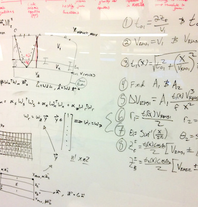
You can see most of the other relationships in this big giant grid I've been slowly chipping away at for ages. Some of it is shown below. It doesn't have most of the P-wave modulus expressions, because no-one seems too bothered about P-wave modulus, despite its obvious resemblance to acoustic impedance. They are in the version on Wikipedia, however (but it lacks the \(V_\mathrm{P}\) and \(V_\mathrm{S}\) expressions).

Some of the expressions for the elastic moduli and velocities — click the image to see them all in SubSurfWiki.

Some of the expressions for the elastic moduli and velocities — click the image to see them all in SubSurfWiki.

In this table, the mysterious quantity \(X\) is given by:

$$ X = \sqrt{9\lambda^2 + 2E\lambda + E^2} $$

In the next post, I'll come back to this grid and tell you how I've been deriving all these equations using Python.


Top tip... To find more posts on rock physics, click the Rock Physics tag below!

Monday highlights from SEG

Ben and I are in New Orleans at the 2015 SEG Annual Meeting, a fittingly subdued affair, given the industry turmoil recently. Lots of people are looking for work, others are thankful to have it.

We ran our annual Geophysics Hackathon over the weekend; I'll write more about that later this week. In a nutshell: despite a low-ish turnout, we had 6 great projects, all of them quite different from anything we've seen before. Once again, Colorado School of Mines dominated.

Beautiful maps

One of the most effective ways to make a tight scientific argument is to imagine trying to convince the most skeptical person you know that your method works. When it comes to seismic attribute analysis, I am that skeptical person.

Some of the nicest images I saw today were in the 'Attributes for Stratigraphic Analysis' session, chaired by Rupert Cole and Yuefeng Sun. For example, Tao Zhao, one of Kurt Marfurt's students, showed some beautiful images from the Waka 3D offshore New Zealand (Zhao & Marfurt). He used 2D colourmaps to co-render two attributes together, along with semblance mapped to opacity on a black layer, and were very nice to look at. However I was left wondering, and not for the first time, how we can do a better job calibrating those maps to geology. We (the interpretation community) need to stop side-stepping that issue; it's central to our credibility. Even if you have no wells, as in this study, you can still use forward models, analogs, or at least interpretation by a sedimentologist, preferably two.

© SEG and Zhao & Marfurt. Left to right: Peak spectral frequency and peak spectral magnitude; GLCM homogeneity; shape index and curvedness. All of the attributes are also corendered with Sobel edge detection.

© SEG and Zhao & Marfurt. Left to right: Peak spectral frequency and peak spectral magnitude; GLCM homogeneity; shape index and curvedness. All of the attributes are also corendered with Sobel edge detection.

Pavel Jilinski at GeoTeric gave a nice talk (Calazans Muniz et al.) about applying some of these sort of fancy displays to a large 3D dataset in Brazil, in a collaboration with Petrobras. The RGB displays of spectral attributes were as expected, but I had not seen their cyan-magenta-yellow (CMY) discontinuity displays before. They map dip to the yellow channel, similarity to the magenta channel, and 'tensor discontinuity' to the cyan channel. No, I don't know what that means either, but the displays were pretty cool.

Publications news

This evening we enjoyed the Editor's Dinner (I coordinate a TLE column and review for Geophysics and Interpretation, so it's totally legit). Good things are coming to the publication world: adopted Canadian Mauricio Sacchi is now Editor-in-Chief, there are no more page charges for colour in Geophysics (up to 10 pages), and watch out for video abstracts next year. Also, Chris Liner mentioned that Interpretation gets 18% of its submissions from oil companies, compared to only 5% for Geophysics. And I heard, but haven't verified, that downturns result in more papers. So at least our journals are healthy. (You do read them, right?)

That's it for today (well, yesterday). More tomorrow!


References

Calazans Muniz, Moises, Thomas Proença, and Pavel Jilinski (2015). Use of Color Blend of seismic attributes in the Exploration and Production Development - Risk Reduction. SEG Technical Program Expanded Abstracts 2015: pp. 1638-1642. doi: 10.1190/segam2015-5916038.1

Zhao, Tao, and Kurt J. Marfurt (2015). Attribute assisted seismic facies classification on a turbidite system in Canterbury Basin, offshore New Zealand. SEG Technical Program Expanded Abstracts 2015: pp. 1623-1627. doi: 10.1190/segam2015-5925849.1

Introducing Bruges

bruges_rooves.png

Welcome to Bruges, a Python library (previously known as agilegeo) that contains a variety of geophysical equations used in processing, modeling and analysing seismic reflection and well log data. Here's what's in the box so far, with new stuff being added every week:


Simple AVO example

VP [m/s] VS [m/s] ρ [kg/m3]
Rock 1 3300 1500 2400
Rock 2 3050 1400 2075

Imagine we're studying the interface between the two layers whose rock properties are shown here...

To compute the zero-offset reflection coefficient at zero offset, we pass our rock properties into the Aki-Richards equation and set the incident angle to zero:

 >>> import bruges as b
 >>> b.reflection.akirichards(vp1, vs1, rho1, vp2, vs2, rho2, theta1=0)
 -0.111995777064

Similarly, compute the reflection coefficient at 30 degrees:

 >>> b.reflection.akirichards(vp1, vs1, rho1, vp2, vs2, rho2, theta1=30)
 -0.0965206980095

To calculate the reflection coefficients for a series of angles, we can pass in a list:

 >>> b.reflection.akirichards(vp1, vs1, rho1, vp2, vs2, rho2, theta1=[0,10,20,30])
 [-0.11199578 -0.10982911 -0.10398651 -0.0965207 ]

Similarly, we could compute all the reflection coefficients for all incidence angles from 0 to 70 degrees, in one degree increments, by passing in a range:

 >>> b.reflection.akirichards(vp1, vs1, rho1, vp2, vs2, rho2, theta1=range(70))
 [-0.11199578 -0.11197358 -0.11190703 ... -0.16646998 -0.17619878 -0.18696428]

A few more lines of code, shown in the Jupyter notebook, and we can make some plots:


Elastic moduli calculations

With the same set of rocks in the table above we could quickly calculate the Lamé parameters λ and µ, say for the first rock, like so (in SI units),

 >>> b.rockphysics.lam(vp1, vs1, rho1), b.rockphysics.mu(vp1, vs1, rho1)
 15336000000.0 5400000000.0

Sure, the equations for λ and µ in terms of P-wave velocity, S-wave velocity, and density are pretty straightforward: 


but there are many other elastic moduli formulations that aren't. Bruges knows all of them, even the weird ones in terms of E and λ.


All of these examples, and lots of others — Backus averaging,  examples are available in this Jupyter notebook, if you'd like to work through them on your own.


Bruges is a...

It is very much early days for Bruges, but the goal is to expose all the geophysical equations that geophysicists like us depend on in their daily work. If you can't find what you're looking for, tell us what's missing, and together, we'll make it grow.

What's a handy geophysical equation that you employ in your work? Let us know in the comments!

Geophysics at SciPy 2015

Yesterday was the geoscience day at SciPy 2015 in Austin.

At lunchtime, Paige Bailey (Chevron) organized a Birds of a Feather on GIS. This was a much-needed meetup for anyone interested in spatial data. It was useful to hear about the tools the fifty-or-so participants  use every day, and a great chance to air some frustrations like Why is it so hard to install a geospatial stack? And questions like How do people make attractive maps with the toolset?

One way to make attractive maps is go beyond the screen and 3D print them. Almost any subsurface dataset could seem more tangible and believable as a 3D object, and Joe Kington (Chevron) showed us how to make data into objects. Just watch:

Matteus Ueckermann followed up with some virtual elevation models, showing how Python can process not just a few tiles of data, but can handle hydrology modeling for the entire world:

Nicola Creati (OGS, Trieste) showed us the PyGmod package, a new and fully parallel geodynamic simulation tool for HPC nuts. So now you can make more plate tectonic models before most people are out of bed!

We also heard from Lindsey Heagy and Gudnir Rosenkjaer from UBC, talking about various applications of Rowan Cockett's awesome SimPEG package to their work. As at the hackathon in Denver, it's very clear that this group's investment in and passion for a well-architected, integrated package is well worth the work, giving everyone who works with it superpowers. And, as we all know, superpowers are awesome. Especially geophysical ones.

Last up, I talked about striplog, a small package for handling interval and point data in logs, core, and other 1D datasets. It's still very immature, but almost ready for real-world users, so if you think you have a use case, I'd love to hear from you.

Today is the last day of the conference part, before we head into the coding sprints tomorrow. Stay tuned for more, or follow the #scipy2015 hashtag to keep up. See all the videos, which go up almost right after talks, on YouTube.

May linkfest

The pick of the links from the last couple of months. We look for the awesome, so you don't have to :)

ICYMI on Pi Day, pimeariver.com wants to check how close river sinuosity comes to pi. (TL;DR — not very.)

If you're into statistics, someone at Imperial College London recently released a nice little app for stochastic simulations of simple calculations. Here's a back-of-the-envelope volumetric calculation by way of example. Good inspiration for our Volume* app.

I love it when people solve problems together on the web. A few days ago Chris Jackson (also at Imperial) posted a question about converting projected coordinates...

I responded with a code snippet that people quickly improved. Chris got several answers to his question, and I learned something about the pyproj library. Open source wins again!

In answering that question, I also discovered that Github now renders most IPython Notebooks. Sweet!

Speaking of notebooks, Beaker looks interesting: individual code blocks support different programming languages within the same notebook and allow you to pass data from one cell to another. For instance, you could do your basic stuff in Python, computationally expensive stuff in Julia, then render a visualization with JavaScript. Here's a simple example from their site.

Python is the language for science, but JavaScript certainly rules the visual side of the web. Taking after JavaScript data-artists like Bret Victor and Mike Bostock, Jack Schaedler has built a fantastic website called Seeing circles, sines, and signals containing visual explanations of signal processing concepts.

If that's not enough for you, there's loads more where that came from: Gallery of Concept Visualization. You're welcome.

My recent notebook about finding small things with 2D seismic grids sparked some chatter on Twitter. People had some great ideas about modeling non-random distributions, like clustered or anisotropic populations. Lots to think about!

Getting help quickly is perhaps social media's most potent capability — though some people do insist on spoiling everything by sharing U might be a genius if u can solve this! posts (gah, stop it!). Earth Science Stack Exchange is still far from being the tool is can be, but there have been some relevant questions on geophysics lately:

A fun thread came up on Reddit too recently: Geophysics software you wish existed. Perfect for inspiring people at hackathons! I'm keeping a list of hacky projects for the next one, by the way.

Not much to say about 3D models in Sketchfab, other than: they're wicked! I mean, check out this annotated anticline. And here's one by R Mahon based on sedimentological experiments by John Shaw and others...

Geocomputing: Call for papers

52 Things .+? Geocomputing is in the works.

For previous books, we've reached out to people we know and trust. This felt like the right way to start our micropublishing project, because we had zero credibility as publishers, and were asking a lot from people to believe anything would come of it.

Now we know we can do it, but personal invitation means writing to a lot of people. We only hear back from about 50% of everyone we write to, and only about 50% of those ever submit anything. So each book takes about 160 invitations.

This time, I'd like to try something different, and see if we can truly crowdsource these books. If you would like to write a short contribution for this book on geoscience and computing, please have a look at the author guidelines. In a nutshell, we need about 600 words before the end of March. A figure or two is OK, and code is very much encouraged. Publication date: fall 2015.

We would also like to find some reviewers. If you would be available to read at least 5 essays, and provide feedback to us and the authors, please let me know

In keeping with past practice, we will be donating money from sales of the book to scientific Python community projects via the non-profit NumFOCUS Foundation.

What the cover might look like. If you'd like to write for us, please read the author guidelines.

What the cover might look like. If you'd like to write for us, please read the author guidelines.

The new open geophysics tools

The hackathon in Denver was more than 6 weeks ago. I kept thinking, "Oh, I must post a review of what went down" (beyond the quick wrap-up I did at the time), but while I'm a firm believer in procrastination six weeks seems unreasonable... Maybe it's taken this long to scrub down to the lasting lessons. Before those, I want to tell you who the teams were, what they did, and where you can find their (100% open source!) stuff. Enjoy!

Geophys Wiz

Andrew Pethick, Josh Poirier, Colton Kohnke, Katerina Gonzales, and Elijah Thomas — GitHub repo

This team had no trouble coming up with ideas — perhaps a reflection of their composition, which was more heterogeneous than the other teams. Josh is at NEOS, the consulting and software firm, and Andrew is a postdoc at Curtin in Perth, Australia, while the other 3 are students at Mines. The team eventually settled on building MT Black Box, a magnetotellurics modeling web application. 

Last thing: Don't miss Andrew Pethick's write-up of the event. 

Seemingly Concerned Neighbours

Elias Arias, Brent Putman, Thomas Rapstine, and Gabriel Martinez — Github repo

These four young geophysicists from the Colorado School of Mines impressed everyone with their work ethic. Their tight-knit team came in with a plan, and proceeded to scribble up the coolest-looking whiteboard of the weekend. After learning some Android development skills 'earlier this week', they pulled together a great little app for forward modeling magnetotelluric responses. 

Hackathon_well_tie_guys.jpg

Well tie guys

Michaël Montouchet, Graham Dawes, Mark Roberts

It was terrific to have pro coders Graham and Michaël with us — they flew from the UK to be with us, thanks to their employer and generous sponsor ffA GeoTeric. They hooked up with Mark, a Denver geophysicist and developer, and hacked on a well-tie web application, rightly identifying a gap in the open source market, so to speak (there is precious little out there for well-based workflows). They may have bitten off more than they could chew in just 2 days, so I hope we can get together with them again to finish it off. Who's up for a European hackathon? 

These two characters from UBC didn't get going till Sunday morning, but in just five hours they built a sweet web app for forward modeling the DC resistivity response of a buried disk. They weren't starting from scratch, because Rowan and others have spent months honing SimPEG, a rich open-source geophysical library, but minds were nonetheless blown.

Key takeaway: interactivity beyond sliders for the win.

Pick This!

Ben Bougher, Jacob Foshee, Evan Bianco, and an immiscible mixture of Chris Chalcraft and me — GitHub repo

Wouldn't you sometimes like to know how other people would interpret the section you're working on? This team, a reprise of the dream team from Houston in 2013, built a simple way to share images and invite others to interpret them. When someone has completed their interpretation, only then do they get to see the ensemble — everyone else's interpretations — in a heatmap. Not only did this team demo live software at pickthis.io, but the audience provided the first crowdsourced picks in real time. 

We'll be blogging more about Pick This soon. We're actively seeking ideas, images, interpreters, and financial support. Keep an eye out.

What I learned at this hackathon

  • Potential fields are an actual thing! OK, kidding, but three out of five teams built potential field modeling tools. I wasn't expecting that, and I think the judges were impressed at the breadth. 
  • 30 hours is easily enough time to build something pretty cool. Heck, 5 hours is enough if you're made of the right stuff. 
  • Students can happily build prototypes alongside professional developers, and even teach them a thing or two. And vice versa. Are hackathons a leveller of playing fields?
  • We need to remove the road blocks to more people enjoying this event. To help with this, next time there will be a 1-day bootcamp before the hackathon.
  • After virtually doubling in size from 2013 to 2014, it's clear that the 2015 Hackathon in New Orleans is going to be awesome! Mark your calendar: 17 and 18 October 2015.

Thank you!

Thank you to the creative, energetic geophysicists that came. It was a privilege to meet and hack with you!

Thank you to the judges who gave up their Sunday teatime to watch the demos and give precious feedback to the teams: Steve Adcock, Jamie Allison, Maitri Erwin, Dennis Cooke, Chris Krohn, Shannon Bjarnason, David Holmes, and Tracy Stark. Amazing people, one and all.

A final Thank You to our sponsors — dGB Earth Sciences, ffA GeoTeric, and OpenGeoSolutions. You guys are totally awesome! Seriously.

sponsors_white_noagile.png

All the time freaks

SEG 2014Thursday was our last day at the SEG Annual Meeting. Evan and I took in the Recent developments in time-frequency analysis workshop, organized by Mirko van der Baan, Sergey Fomel, and Jean-Baptiste Tary (Vienna). The workshop came out of an excellent paper I reviewed this summer, which was published online a couple of weeks ago:

Tary, JB, RH Herrera, J Han, and M van der Baan (2014), Spectral estimation—What is new? What is next?, Rev. Geophys. 52. doi:10.1002/2014RG000461.

The paper compares the results of several time–frequency transforms on a suite of 'benchmark' signals. The idea of the workshop was to invite further investigation or other transforms. The organizers did a nice job of inviting contributors with diverse interests and backgrounds. The following people gave talks, several of them sharing their code (*):

  • John Castagna (Lumina) with a review of the applications of spectral decomposition for seismic analysis.
  • Steven Lin (NCU, Taiwan) on empirical methods and the Hilbert–Huang transform.
  • Hau-Tieng Wu (Toronto) on the application of transforms to monitoring respiratory patterns in animals.*
  • Marcílio Matos (SISMO) gave an entertaining, talk about various aspects of the problem.
  • Haizhou Yang (Standford) on synchrosqueezing transforms applied to problems in anatomy.*
  • Sergey Fomel (UT Austin) on Prony's method... and how things don't always work out.*
  • Me, talking about the fidelity of time–frequency transforms, and some 'unsolved problems' (for me).*
  • Mirko van der Baan (Alberta) on the results from the Tary et al. paper.

Some interesting discussion came up in the two or three unstructured parts of the session, organized as mini-panel discussions with groups of authors. Indeed, it felt like the session could have lasted longer, because I don't think we got very close to resolving anything. Some of the points I took away from the discussion:

  • My observation: there is no existing survey of the performance of spectral decomposition (or AVO) — these would be great risking tools.
  • Castagna's assertion: there is no model that predicts the low-frequency 'shadow' effect (confusingly it's a bright thing, not a shadow).
  • There is no agreement on whether the so-called 'Gabor limit' of time–frequency localization is a lower-bound on spectral decomposition. I will write more about this in the coming weeks.
  • Should we even be attempting to use reassignment, or other 'sharpening' tools, on broadband signals? To put it another way: does instantaneous frequency mean anything in seismic signals?
  • What statistical measures might help us understand the amount of reassignment, or the precision of time–frequency decompositions in general?

The fidelity of time–frequency transforms

My own talk was one of the hardest I've ever done, mainly because I don't think about these problems very often. I'm not much of a mathematician, so when I do think about them, I tend to have more questions than insights, so I made my talk into a series of questions for the audience. I'm not sure I got much closer to any answers, but I have a better idea of my questions now... which is a kind of progress I suppose.

Here's my talk (latest slidesGitHub repo). Comments and feedback are, as always, welcome.


SEG 2014: sampling from the smorgasbord

Next week, Matt and I will be attending the 2014 SEG Annual General Meeting at the Colorado Convention Centre in Denver. Join the geo-tweeting using the hashtag #SEG2014 and stay tuned on the blog for our daily highlights.

Fitness training

I spent a couple of hours yesterday reviewing the conference schedule in an attempt to form an opinion on what deserved my attention. The meeting boasts content from over 1600 abstract submissions which it has dispersed over three formats: oral presentations, poster presentations, and oral discussions/e-posters (looking forward to finding out how these work). Any given moment there will be 12 oral, 3 poster, and 6 e-poster presentations going on, not to mention all the happenings on the exhibition floor. A worthy test for my navigation skills, discipline, and endurance, as well as the new and improved SEG events mobile app.

The technical program

There are 101 sessions in the technical program, each with around 8 presentations. Six of these sessions are dubbed special sessions, hosting either invited speakers from other domains such as hydrogeophysics and completions engineering, or a heavyweight lineup of seismic celebs. Special session numero uno, entitled Recent Advances And The Road Ahead is  the session that I'm most looking forward to. It kicks off the technical program on Monday afternoon with talks from:

  • Christof Stork (ION Geophysical), The decline of conventional seismic acquisition and the rise of specialized acquisition: this is compressive sensing.
  • Sergy Fomel (UT Austin), Recent advances in time-domain seismic imaging. 
  • John Etgen (BP), Seismic adaptive optics. 
  • Kurt Marfurt (Univ. of Oklahoma), Seismic attributes and the road ahead. 
  • Reinarldo Michelena (iReservoir), Flow simulation models for unconventional reservoirs: The role of seismic data.

Other presentations throughout the week that have made it onto my must-see list:

  • Andreas Rüger (Halliburton), A practitioner's approach to full waveform inversion.
  • Lewis Li (Stanford), Uncertainty maps for seismic images through geostatistical model randomization.
  • Kevin Liner (Univ. of Arkansas), Study of basement rocks in Northeastern Oklahoma with 3D seismic and well logs.
  • Xinyuan Luan (China Univ. of Petroleum), Laboratory measurements of brittleness anisotropy in synthetic shale with different cementation.
  • Anya Reitz (Colorado School of Mines), Feasibility of surface and borehole time-lapse gravity for SAGD monitoring.
  • Cai Lu (Univ. of Electronic Science and Technology of China), Application of multi-attributes fused volume rendering techniques in 3D seismic interpretation.

To top it all off on Thursday afternoon, Matt and I will be at workshop number 9, Latest Developments in Time-Frequency Analysis. It is one of many post convention workshops worth sticking around for after the booths get torn down and the the exhibition doors close.

SEG Wikithon

If you read The Leading Edge frequently or if you visit the SEG website regularly, you may have noticed an increased presence of SEG Wiki. Matt and his allies Isaac Farley and Andrew Geary will be parked in Room 708 between 12–2pm and 5–6pm October 26–29. For more information about SEG Wiki and the Wikithon, check out Isaac's article from the September issue, and find out all the details on wiki page (naturally).

Whatever you want to call it

Lastly, I couldn't help but snag a selection of the coolest names from the technical session. I can only imagine what the organizing committee was thinking:

Well, they got my attention. And with so much content to choose from, maybe that's all that matters.

Image by user bonjourpeewee on flickr, licensed CC-BY-SA.

The hackathon is coming

The Geophysics Hackathon is one month away! Signing up is not mandatory — you can show up on the day if you like — but it does help with the planning. It's 100% free, and I guarantee you'll enjoy yourself. You'll also learn tons about geophysics and about building software. Deets: Thrive, Denver, 8 am, 25–26 October. Bring a laptop.

Need more? Here's all the info you could ask for. Even more? Ask by email or in the comments

Send your project ideas

The theme this year is RESOLUTION. Participants are encouraged to post projects to hackathon.io ahead of time — especially if you want to recruit others to help. And even if you're not coming to the event, we'd love to hear your project ideas. Here are some of the proto-ideas we have so far: 

  • Compute likely spatial and temporal resolution from some basic acquisition info: source, design, etc.
  • Do the same but from information from the stack: trace spacing, apparent bandwidth, etc.
  • Find and connect literature about seismic and log resolution using online bibliographic data.
  • What does the seismic spectrum look like, given STFT limitations, or Gabor uncertainty?

If you have a bright idea, get in touch by email or in the comments. We'd love to hear from you.

Thank you to our sponsors

Three forward-thinking companies have joined us in making the hackathon as much a geophysics party as well as a scientific workshop (a real workshop). I think this industry may have trained us to take event sponsorship for granted, but it's easy to throw $5000 at the Marriott for Yet Another Coffee Break. Handing over money to a random little company in Nova Scotia to buy coffee, tacos, and cool swag for hungry geophysicists and programmers takes real guts! 

Please take a minute to check out our sponsors and reward them for supporting innovation in our community. 

dGB GeoTeric OGS

Students: we are offering $250 bursaries to anyone looking for help with travel or accommodation. Just drop me a line with a project idea. If you know a student that might enjoy the event, please forwadrd this to them.