Deriving equations in Python

Last week I wrote about the elastic moduli, and showed the latest version of my table of equations. Here it is; click on it for a large version:

View fullsize

Making this grid was a bit of an exercise in itself. One could spend some happy hours rearranging things by hand; instead, I spent some (mostly) happy hours learning to use SymPy, a symbolic maths library for Python. For what it's worth, you can see my flailing in this Jupyter Notebook. Warning: it's pretty untidy.

Wrangling equations

Fortunately, SymPy is easy to get started with. Let's look at getting an expression for \(V_\mathrm{P}\) in terms of \(E\) and \(K\), given that I already have an expression in terms of \(E\) and \(\mu\), plus an expression for \(\mu\) in terms of \(E\) and \(K\).

First we import the SymPy library, set it up for nice math display in the Notebook, and initialize some parameter names:

>>> import sympy
>>> sympy.init_printing(use_latex='mathjax')
>>> lamda, mu, nu, E, K, rho = sympy.symbols("lamda, mu, nu, E, K, rho")

lamda is not a typo: lambda means something else in Python — it's a sort of unnamed function.

Now we're ready to define an expression. First, I'll import SymPy's own square root function for convenience. Then I define an expression for \(V_\mathrm{P}\) in terms of \(E\) and \(\mu\):

>>> vp_expr = sympy.sqrt((mu * (E - 4*mu)) / (rho * (E - 3*mu)))
>>> vp_expr

$$ \sqrt{\frac{\mu \left(E - 4 \mu\right)}{\rho \left(E - 3 \mu\right)}} $$

Now we can give SymPy the expression for \(\mu\) in terms of \(E\) and \(K\) and substitute:

>>> mu_expr = (3 * K * E) / (9 * K - E)
>>> vp_new = vp_expr.subs(mu, mu_expr)
>>> vp_new

$$\sqrt{3} \sqrt{\frac{E K \left(- \frac{12 E K}{- E + 9 K} + E\right)}{\rho \left(- E + 9 K\right) \left(- \frac{9 E K}{- E + 9 K} + E\right)}}$$

Argh, what is that?? Luckily, it's easy to simplify:

>>> sympy.simplify(vp_new)

$$\sqrt{3} \sqrt{\frac{K \left(E + 3 K\right)}{\rho \left(- E + 9 K\right)}}$$

That's more like it! What's really cool is that SymPy can even generate the \(\LaTeX\) code for your favourite math renderer:

>>> print(sympy.latex(sympy.simplify(vp_new)))
\sqrt{3} \sqrt{\frac{K \left(E + 3 K\right)}{\rho \left(- E + 9 K\right)}}

That's all there is to it!

What is the mystery X?

Have a look at the expression for  \(V_\mathrm{P}\) in terms of \(E\) and \(\lambda\):

$$\frac{\sqrt{2}}{2} \sqrt{\frac{1}{\rho} \left(E - \lambda + \sqrt{E^{2} + 2 E \lambda + 9 \lambda^{2}}\right)}$$

I find this quantity — I call it \(X\) in the big table of equations — really curious:

$$ X = \sqrt{9\lambda^2 + 2E\lambda + E^2} $$

As you can see from the similar table on Wikipedia, a similar quantity appears in expressions in terms of \(E\) and \(M\). These quantities look like elastic moduli, and even have the right units and order of magnitude as the others. If anyone has thoughts on what significance it might have, if any, or on why expressions in terms of \(E\) and \(\lambda\) or \(M\) should be so uncommonly clunky, I'm all ears. 

One last thing... I've mentioned Melvyn Bragg's wonderful BBC radio programme In Our Time before. If you like listening to the radio, try this recent episode on the life and work of Robert Hooke. Not only did he invent the study of elasticity with his eponymous law, he was also big in microscopy, describing things like the cellular structure of cork in detail (right).

All the elastic moduli

An elastic modulus is the ratio of stress (pressure) to strain (deformation) in an isotropic, homogeneous elastic material:

$$ \mathrm{modulus} = \frac{\mathrm{stress}}{\mathrm{strain}} $$

OK, what does that mean?

Elastic means what you think it means: you can deform it, and it springs back when you let go. Imagine stretching a block of rubber, like the picture here. If you measure the stress \(F/W^2\) (i.e. the pressure is force per unit of cross-sectional area) and strain \(\Delta L/L\) (the stretch as a proportion) along the direction of stretch ('longitudinally'), then the stress/strain ratio gives you Young's modulus, \(E\).

Since strain is unitless, all the elastic moduli have units of pressure (pascals, Pa), and is usually on the order of tens of GPa (billions of pascals) for rocks. 

The other elastic moduli are: 

• Shear modulus, \(\mu\) or \(G\), a measure of shear elasticity.

• 1st Lamé parameter, \(\lambda\), which famously 'has no physical interpretation'. I bet Bill Goodway would disagree: he calls \(\lambda\) "a pure, unambiguous and true measure of incompressibility, as it relates normal axial and lateral strain to uniaxial normal stress" (CSEG Recorder, June 2014).

• Bulk modulus, \(K\) a measure of volumetric elasticity.

• P-wave modulus, \(M\), a measure of longitudinal elasticity that shows up — as \(\lambda + 2\mu\) — all over the place in seismology, for example in the isotropic elastic wave equation. Still, it doesn't get a lot of love.

There's another quantity that doesn't fit our definition of a modulus, and doesn't have units of pressure — in fact it's unitless —  but is always lumped in with the others: 

• Poisson's ratio, \(\nu\), the ratio of transverse to longitudinal strain.

View fullsize

What does this have to do with my data?

Interestingly, and usefully, the elastic properties of isotropic materials are described completely by any two moduli. This means that, given any two, we can compute all of the others. More usefully still, we can also relate them to \(V_\mathrm{P}\), \(V_\mathrm{S}\), and \(\rho\). This is great because we can get at those properties easily via well logs and less easily via seismic data. So we have a direct path from routine data to the full suite of elastic properties.

The only way to measure the elastic moduli themselves is on a mechanical press in the laboratory. The rock sample can be subjected to confining pressures, then squeezed or stretched along one or more axes. There are two ways to get at the moduli:

1. Directly, via measurements of stress and strain, so called static conditions.

2. Indirectly, via sonic measurements and the density of the sample. Because of the oscillatory and transient nature of the sonic pulses, we call these dynamic measurements. In principle, these should be the most comparable to the measurements we make from well logs or seismic data.

Let's see the equations then

The elegance of the relationships varies quite a bit. Shear modulus \(\mu\) is just \(\rho V_\mathrm{S}^2\), but Young's modulus is not so pretty:

$$ E = \frac{\rho V_\mathrm{S}^2 (3 V_\mathrm{P}^2 - 4 V_\mathrm{S}^2) }{V_\mathrm{P}^2 - V_\mathrm{S}^2} $$

You can see most of the other relationships in this big giant grid I've been slowly chipping away at for ages. Some of it is shown below. It doesn't have most of the P-wave modulus expressions, because no-one seems too bothered about P-wave modulus, despite its obvious resemblance to acoustic impedance. They are in the version on Wikipedia, however (but it lacks the \(V_\mathrm{P}\) and \(V_\mathrm{S}\) expressions).

Some of the expressions for the elastic moduli and velocities — click the image to see them all in SubSurfWiki.

In this table, the mysterious quantity \(X\) is given by:

$$ X = \sqrt{9\lambda^2 + 2E\lambda + E^2} $$

In the next post, I'll come back to this grid and tell you how I've been deriving all these equations using Python.

---

Top tip... To find more posts on rock physics, click the Rock Physics tag below!

All the time freaks

Thursday was our last day at the SEG Annual Meeting. Evan and I took in the Recent developments in time-frequency analysis workshop, organized by Mirko van der Baan, Sergey Fomel, and Jean-Baptiste Tary (Vienna). The workshop came out of an excellent paper I reviewed this summer, which was published online a couple of weeks ago:

Tary, JB, RH Herrera, J Han, and M van der Baan (2014), Spectral estimation—What is new? What is next?, Rev. Geophys. 52. doi:10.1002/2014RG000461.

The paper compares the results of several time–frequency transforms on a suite of 'benchmark' signals. The idea of the workshop was to invite further investigation or other transforms. The organizers did a nice job of inviting contributors with diverse interests and backgrounds. The following people gave talks, several of them sharing their code (*):

• John Castagna (Lumina) with a review of the applications of spectral decomposition for seismic analysis.
• Steven Lin (NCU, Taiwan) on empirical methods and the Hilbert–Huang transform.
• Hau-Tieng Wu (Toronto) on the application of transforms to monitoring respiratory patterns in animals.*
• Marcílio Matos (SISMO) gave an entertaining, talk about various aspects of the problem.
• Haizhou Yang (Standford) on synchrosqueezing transforms applied to problems in anatomy.*
• Sergey Fomel (UT Austin) on Prony's method... and how things don't always work out.*
• Me, talking about the fidelity of time–frequency transforms, and some 'unsolved problems' (for me).*
• Mirko van der Baan (Alberta) on the results from the Tary et al. paper.

Some interesting discussion came up in the two or three unstructured parts of the session, organized as mini-panel discussions with groups of authors. Indeed, it felt like the session could have lasted longer, because I don't think we got very close to resolving anything. Some of the points I took away from the discussion:

• My observation: there is no existing survey of the performance of spectral decomposition (or AVO) — these would be great risking tools.
• Castagna's assertion: there is no model that predicts the low-frequency 'shadow' effect (confusingly it's a bright thing, not a shadow).
• There is no agreement on whether the so-called 'Gabor limit' of time–frequency localization is a lower-bound on spectral decomposition. I will write more about this in the coming weeks.
• Should we even be attempting to use reassignment, or other 'sharpening' tools, on broadband signals? To put it another way: does instantaneous frequency mean anything in seismic signals?
• What statistical measures might help us understand the amount of reassignment, or the precision of time–frequency decompositions in general?

The fidelity of time–frequency transforms

My own talk was one of the hardest I've ever done, mainly because I don't think about these problems very often. I'm not much of a mathematician, so when I do think about them, I tend to have more questions than insights, so I made my talk into a series of questions for the audience. I'm not sure I got much closer to any answers, but I have a better idea of my questions now... which is a kind of progress I suppose.

Here's my talk (latest slides — GitHub repo). Comments and feedback are, as always, welcome.

Great geophysicists #12: Gauss

Carl Friedrich Gauss was born on 30 April 1777 in Braunschweig (Brunswick), and died at the age of 77 on 23 February 1855 in Göttingen. He was a mathematician, you've probably heard of him; he even has his own Linnean handle: Princeps mathematicorum, or Prince of mathematicians (I assume it's the royal kind, not the Purple Rain kind — ba dum tss).

Gauss's parents were poor, working class folk. I wonder what they made of their child prodigy, who allegedly once stunned his teachers by summing the integers up to 100 in seconds? At about 16, he was quite a clever-clogs, rediscovering Bode's law, the binomial theorem, and the prime number theorem. Ridiculous.

His only imperfection was that he was too much of a perfectionist. His motto was pauca sed matura, meaning "few, but ripe". It's understandable how someone so bright might not feel much need to share his work, but historian Eric Temple Bell reckoned that if Gauss had published his work regularly, he would have advanced mathematics by fifty years.

He was only 6 when Euler died, but surely knew his work. Euler is the only other person who made comparably broad contributions to what we now call the exploration geophysics toolbox, and applied physics in general. Here are a few: 

• He proved the fundamental theorems of algebra and arithmetic. No big deal.
• He formulated the Gaussian function — which of course crops up everywhere, especially in geostatistics. The Ricker wavelet is a pulse with frequencies distributed in a Gaussian.
• The gauss is the cgs unit of magnetic flux density, thanks to his work on the flux theorem, one of Maxwell's equations.
• He discovered the Cauchy integral theorem for contour integrals but did not publish it.
• The 'second' or 'total' curvature — a coordinate-system-independent measure of spatial curvedness — is named after him.
• He made discoveries in non-Euclidean geometry, but did not publish them.

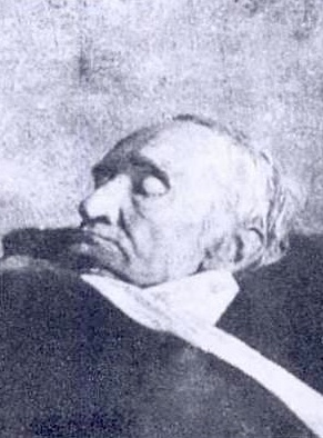
Excitingly, Gauss is the first great geophysicist we've covered in this series to have been photographed (right). Unfortunately, he was already dead. But what an amazing thing, to peer back through time almost 160 years.

Next time: Augustin-Jean Fresnel, a pioneer of wave theory.

Well tie calculus

As Matt wrote in March, he is editing a regular Tutorial column in SEG's The Leading Edge. I contributed the June edition, entitled Well-tie calculus. This is a brief synopsis only; if you have any questions about the workflow, or how to get started in Python, get in touch or come to my course.

---

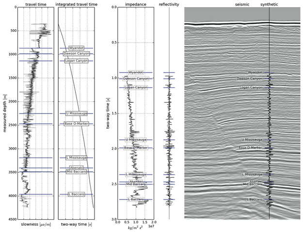
Synthetic seismograms can be created by doing basic calculus on traveltime functions. Integrating slowness (the reciprocal of velocity) yields a time-depth relationship. Differentiating acoustic impedance (velocity times density) yields a reflectivity function along the borehole. In effect, the integral tells us where a rock interface is positioned in the time domain, whereas the derivative tells us how the seismic wavelet will be scaled.

This tutorial starts from nothing more than sonic and density well logs, and some seismic trace data (from the #opendata Penobscot dataset in dGB's awesome Open Seismic Repository). It steps through a simple well-tie workflow, showing every step in an IPython Notebook:

1. Loading data with the brilliant LASReader
2. Dealing with incomplete, noisy logs
3. Computing the time-to-depth relationship
4. Computing acoustic impedance and reflection coefficients
5. Converting the logs to 2-way travel time
6. Creating a Ricker wavelet
7. Convolving the reflection coefficients with the wavelet to get a synthetic
8. Making an awesome plot, like so...

Final thoughts

If you find yourself stretching or squeezing a time-depth relationship to make synthetic events align better with seismic events, take the time to compute the implied corrections to the well logs. Differentiate the new time-depth curve. How much have the interval velocities changed? Are the rock properties still reasonable? Synthetic seismograms should adhere to the simple laws of calculus — and not imply unphysical versions of the earth.

---

Matt is looking for tutorial ideas and offers to write them. Here are the author instructions. If you have an idea for something, please drop him a line.

Fitting a model to data

In studying the earth, we can't afford to take enough observations, and they will never be free of noise. So if you say you do geoscience, I hereby challenge you to formulate your work as a mathematical inverse problem. Inversion is a question: given the data, the physical equations, and details of the experiment, what is the distribution of physical properties? To answer this question we must address three more fundamental ones (Scales, Smith, and Treitel, 2001):

• How accurate is the data? Or what does fit mean?
• How accurately can we model the response of the system? Have we included all the physics that can contribute signifcantly to the data?
• What is known about the system independent of the data? There must be a systematic procedure for rejecting unreasonable models that fit the data as well.

Setting up an inverse problem means coming up with the equations that contain the physics and geometry of the system under study. The method for solving it depends on the nature of the system of equations. The simplest is the minimum norm solution, and you've heard of it before, but perhaps under a different name.

To fit is to optimize a system of equations

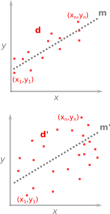
For problems where the number of observations is greater than the number of unknowns, we want to find which unknowns fit the best. One case you're already familiar with is the method of least squares — you've used it fitting a line of through a set of points. A line is unambiguously described by only two parameters: slope a and y-axis intercept b. These are the unknowns in the problem, they are the model m that we wish to solve for. The problem of line-fitting through a set of points can be written out like this,

As I described in a previous post, the system of the problem takes the form d = Gm, where each row links a data point to an equation of a line. The model vector m (M × 1), is smaller than the data d (N × 1) which makes it an over-determined problem, and G is a N × M matrix holding the equations of the system.

Why cast a system of equations in this matrix form? Well, it turns out that the the best-fit line is precisely,

which are trivial matrix operations, once you've written out G.  T means to take the transpose, and –1 means the inverse, the rest is matrix multiplication. Another name for this is the minimum norm solution, because it defines the model parameters (slope and intercept) for which the lengths (vector norm) between the data and the model are a minimum. 

One benefit that comes from estimating a best-fit model is that you get the goodness-of-fit for free. Which is convenient because making sense of the earth doesn't just mean coming up with models, but also expressing their uncertainty, in terms of the errors with which they are linked.

I submit to you that every problem in geology can be formulated as a mathematical inverse problem. The benefit of doing so is not just to do math for math's sake, but it is only through quantitatively portraying ambiguous inferences and parameterizing non-uniqueness that we can do better than interpreting or guessing. 

Reference (well worth reading!)

Scales, JA, Smith, ML, and Treitel, S (2001). Introductory Geophysical Inverse Theory. Golden, Colorado: Samizdat Press. 

Backwards and forwards reasoning

Most people, if you describe a train of events to them will tell you what the result will be. There will be few people however, that if you told them a result, would be able to evolve from their own consciousness what the steps were that led to that result. This is what I mean when I talk about reasoning backward.

— Sherlock Holmes, A Study in Scarlet, Sir Arthur Conan Doyle (1887)

Reasoning backwards is the process of solving an inverse problem — estimating a physical system from indirect data. Straight-up reasoning, which we call the forward problem, is a kind of data collection: empiricism. It obeys a natural causality by which we relate model parameters to the data that we observe.

Modeling a measurement

Where are you headed? Every subsurface problem can be expressed as the arrow between two or more such panels.Inverse problems exists for two reasons. We are incapable of measuring what we are actually interested in, and it is impossible to measure a subject in enough detail, and in all aspects that matter. If, for instance, I ask you to determine my weight, you will be troubled if the only tool I allow is a ruler. Even if you are incredibly accurate with your tool, at best, you can construct only an estimation of the desired quantity. This estimation of reality is what we call a model. The process of estimation is called inversion.

Measuring a model

Forward problems are ways in which we acquire information about natural phenomena. Given a model (me, say), it is easy to measure some property (my height, say) accurately and precisely. But given my height as the starting point, it is impossible to estimate the me from which it came. This is an example of an ill-posed problem. In this case, there is an infinite number of models that share my measurements, though each model is described by one exact solution. 

Solving forward problems are nessecary to determine if a model fits a set of observations. So you'd expect it to be performed as a routine compliment to interpretation; a way to validate our assumptions, and train our intuition.  

The math of reasoning

Forward and inverse problems can be cast in this seemingly simple equation.

where d is a vector containing N observations (the data), m is a vector of M model parameters (the model), and G is a N × M matrix operator that connects the two. The structure of G changes depending on the problem, but it is where 'the experiment' goes. Given a set of model parameters m, the forward problem is to predict the data d produced by the experiment. This is as simple as plugging values into a system of equations. The inverse problem is much more difficult: given a set of observations d, estimate the model parameters m.

I think interpreters should describe their work within the Gm = d framework. Doing so would safeguard against mixing up observations, which should be objective, and interpretations, which contain assumptions. Know the difference between m and d. Express it with an arrow on a diagram if you like, to make it clear which direction you are heading in.

Illustrations for this post were created using data from the Marmousi synthetic seismic data set. The blue seismic trace and its corresponding velocity profile is at location no. 250.

How to get paid big bucks

Yesterday I asked 'What is inversion?' and started looking at problems in geoscience as either forward problems or inverse problems. So what are some examples of inverse problems in geoscience? Reversing our forward problem examples:

• Given a suite of sedimentological observations, provide the depositional environment. This is a hard problem, because different environments can produce similar-looking facies. It is ill-conditioned, because small changes in the input (e.g. the presence of glaucony, or Cylindrichnus) produces large changes in the interpretation.
• Given a seismic trace, produce an impedance log. Without a wavelet, we cannot uniquely deduce the impedance log — there are infinitely many combinations of log and wavelet that will give rise to the same seismic trace. This is the challenge of seismic inversion. 

To solve these problems, we must use induction — a fancy name for informed guesswork. For example, we can use judgement about likely wavelets, or the expected geology, to constrain the geophysical problem and reduce the number of possibilities. This, as they say, is why we're paid the big bucks. Indeed, perhaps we can generalize: people who are paid big bucks are solving inverse problems...

• How do we balance the budget?
• What combination of chemicals might cure pancreatic cancer?
• What musical score would best complement this screenplay?
• How do I act to portray a grief-stricken war veteran who loves ballet?

What was the last inverse problem you solved?

Update on 2013-04-17 21:50 by Matt Hall

Moar inversion! Don't miss the previous post in this mini-series, or the next one — where things get a bit more mathy. 

What is inversion?

Inverse problems are at the heart of geoscience. But I only hear hardcore geophysicists talk about them. Maybe this is because they're hard problems to solve, requiring mathematical rigour and computational clout. But the language is useful, and the realization that some problems are just damn hard — unsolvable, even — is actually kind of liberating. 

Forwards first

Before worrying about inverse problems, it helps to understand what a forward problem is. A forward problem starts with plenty of inputs, and asks for a straightforward, algorithmic, computable output. For example:

• What is 4 × 5?
• Given a depositional environment, what sedimentological features do we expect?
• Given an impedance log and a wavelet, compute a synthetic seismogram.

These problems are solved by deductive reasoning, and have outcomes that are no less certain than the inputs.

Can you do it backwards?

You can guess what an inverse problem looks like. Computing 4 × 5 was pretty easy, even for a geophysicist, but it's not only difficult to do it backwards, it's impossible:

20 = what × what

You can solve it easily enough, but solutions are, to use the jargon, non-unique: 2 × 10, 7.2 × 1.666..., 6.3662 × π — you get the idea. One way to deal with such under-determined systems of equations is to know about, or guess, some constraints. For example, perhaps our system — our model — only includes integers. That narrows it down to three solutions. If we also know that the integers are less than 10, there can be only one solution.

Non-uniqueness is a characteristic of ill-posed problems. Ill-posedness is a dead giveaway of an inverse problem. Proposed by Jacques Hadamard, the concept is the opposite of well-posedness, which has three criteria:

• A solution exists.
• The solution is unique.
• The solution is well-conditioned, which means it doesn't change disproportionately when the input changes. 

Notice the way the example problem was presented: one equation, two unknowns. There is already a priori knowledge about the system: there are two numbers, and the operator is multiplication. In geoscience, since the earth is not a computer, we depend on such knowledge about the nature of the system — what the variables are, how they interact, etc. We are always working with a model of nature.

Tomorrow, I'll look at some specific examples of inverse problems, and Evan will continue the conversation next week.

Update on 2013-04-12 11:18 by Matt Hall

Don't miss the first follow-up to this article, How to get paid big bucks. 

Cross plots: a non-answer

On Monday I asked whether we should make crossplots according to statistical rules or natural rules. There was some fun discussion, and some awesome computation from Henry Herrera, and a couple of gems:

Physics likes math, but math doesn't care about physics — @jeffersonite

But... when I consider the intercept point I cannot possibly imagine a rock that has high porosity and zero impedance — Matteo Niccoli, aka @My_Carta

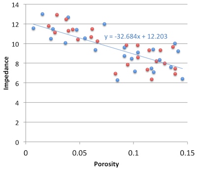
I tried asking on Stack Overflow once, but didn’t really get to the bottom of it, or perhaps I just wasn't convinced. The consensus seems to be that the statistical answer is to put porosity on y-axis, because that way you minimize the prediction error on porosity. But I feel—and this is just my flaky intuition talking—like this fails to represent nature (whatever that means) and so maybe that error reduction is spurious somehow.

Reversing the plot to what I think of as the natural, causation-respecting plot may not be that unreasonable. It's effectively the same as reducing the error on what was x (that is, impedance), instead of y. Since impedance is our measured data, we could say this regression respects the measured data more than the statistical, non-causation-respecting plot.

So must we choose? Minimize the error on the prediction, or minimize the error on the predictor. Let's see. In the plot on the right, I used the two methods to predict porosity at the red points from the blue. That is, I did the regression on the blue points; the red points are my blind data (new wells, perhaps). Surprisingly, the statistical method gives an RMS error of 0.034, the natural method 0.023. So my intuition is vindicated! 

Unfortunately if I reverse the datasets and instead model the red points, then predict the blue, the effect is also reversed: the statistical method does better with 0.029 instead of 0.034. So my intuition is wounded once more, and limps off for an early bath.

Irreducible error?

Here's what I think: there's an irreducible error of prediction. We can beg, borrow or steal error from one variable, but then it goes on the other. It's reminiscent of Heisenberg's uncertainty principle, but in this case, we can't have arbitrarily precise forecasts from imperfectly correlated data. So what can we do? Pick a method, justify it to yourself, test your assumptions, and then be consistent. And report your errors at every step. 

I'm reminded of the adage 'Correlation does not equal causation.' Indeed. And, to borrow @jeffersonite's phrase, it seems correlation also does not care about causation.