Fabric facies

I set out to detect patterns in images, with the conviction that they are diagnostic of more telling physical properties of the media. Tea towel textures can indicate absorbency, durability, state of wear and tear, etc. Seismic textures can indicate things like depositional environment, degree of deformation, lithologic content, and so on:

Facies: A rock or stratified body distinguished from others by its appearance or composition.

Facies are clusters distinguishable in all visual media. Geophysicists shouldn't be afraid of using the word normally reserved by geologists—seismic facies. In the seismic case, instead of lithology, grain size, bedding patterns, and so on, we are using attributes such as amplitude, energy, coherency, and Haralick textures for classification.

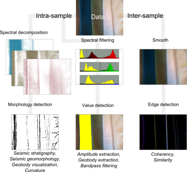
The brain is good at pattern recognition and picking out subtleties. I can assign facies to the input data (A), based on on hues (B), or patterns (C). I can also count objects (D), interpret boundaries (E), and identify poorly resolved regions of an image (F) caused by shadows or noise. I can even painstakingly draw the pockmarks or divets in the right hand teatowel (G). All of these elements can be simultaneously held in the mind of the viewer and comprise what we naturally perceive as the properties of visual media. Isolating, extracting, and illustrating these visual features by hand remains tedious.

I am not interested in robot vision so computers can replace geophysical interpreters, but I am interested in how image classification can be used to facilitate, enrich, and expedite the interpretive process. You can probably already think of attributes we can use to coincide with this human interpretation from the examples I gave in a previous post.

Identifying absorbency

Let's set an arbitrary goal of classifying the ability to soak up water, or absorbency. Surely a property of interest to anyone studying porous media. Because absorbency is a media-property, not an optical property (like colour) or a boundary property (like edges), it makes sense to use texture classification. From the input image, I can count 5 different materials, each with a distinct pattern. The least tractable might be the rightmost fabric which has alternating waffle-dimple segments, troublesome shadows and contours, and patterns at two different scales. The test of success is seeing how this texture classification compares to the standard approach of visual inspection and manual picking. 

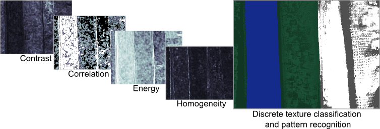
I landed on using 7 classes for this problem. Two for the white tea-towels, two for the green tea-towel, one for the blue, and one that seems to be detecting shadows (shown in dark grey). Interestingly, the counter top on the far left falls into the same texture class as the green tea-towel. Evidence that texture alone isn't a foolproof proxy for absorbency. To improve the classification, I would need to allow more classes (likely 8 or 9). 

It seems to me that the manual picks match the classification quite well. The picks lack detail, as with any interpretation, but they also lack noise. On the contrary, there are some locations where the classification has failed. It stuggles in low-light and over-exposed regions. 

If you are asking, "is one approach better than the other?", you are asking the wrong question. These are not mutually exclusive approaches. The ideal scenario is one which uses these methods in concert for detecting geologic features in the fabric of seismic data. 

Fabric textures

Beyond the traditional, well-studied attributes that I referred to last time, are a large family of metrics from image processing and robot vision. The idea is to imitate the simple pattern recognition rules our brains intuitively and continuously apply when we look at seismic data: how do the data look? How smooth or irregular are the reflections? If you thought the adjectives I used for my tea towels were ambiguous, I assure you seismic will be much more cryptic.

In three-dimensional data, texture is harder to see, difficult to draw, and impossible to put on a map. So when language fails us, discard words altogether and use numbers instead. While some attributes describe the data at a particular place (as we might describe a photographic pixel as 'red', 'bright', 'saturated'), other attributes describe the character of the data in a small region or kernel ('speckled', 'stripy', 'blurry').

Texture by numbers

I converted the colour image from the previous post to a greyscale image with 256 levels (a bit-depth of 8) to match this notion of scalar seismic data samples in space. The geek speak is that I am computing local grey-level co-occurence matrices (or GLCMs) in a moving window around the image, and then evaluating some statistics of the local GLCM for each point in the image. These statistics are commonly called Haralick textures. Choosing the best kernel size will depend on the scale of the patterns. The Haralick textures are not particularly illustrative when viewed on their own but they can be used for data clustering and classification, which will be the topic of my next post.

• Step 1: Reduce the image to 256 grey-levels
• Step 2: For every pixel, compute a co-occurrence matrix from a p by q kernel (p, q = 15 for my tea towel photo)
• Step 3: For every pixel, compute the Haralick textures (Contrast, Correlation, Energy, Homogeneity) from the GLCM

Textures in seismic data

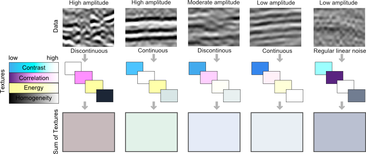
Here are a few tiles of seismic textures that I have loosely labeled as "high-amplitude continous", "high-amplitude discontinuous", "low-amplitude continuous", etc. You certainly might choose different words to describe them, but each has a unique and objective set of Haralick textures. I have explicitly represented the value of each's texture as a color; using cyan for contrast, magenta for correlation, yellow for energy, and black for homogeneity. Thus, the four Haralick textures span the CMYK color space. Merging these components back together into a single color gives you a sense of the degree of difference across the tiles. For instance, the high-amplitude continuous tile, is characterized by high contrast and high energy, but low correlation, relative to the low-amplitude continuous tile. Their textures are similar, so obviously, they map to similar color values in CMYK color space. Whether or not they are truly discernable is the challenge we offer to data clustering; be it employed by visual inspection or computational force.

Further reading:
Gao, D., 2003, Volume texture extraction for 3D seismic visualization and interpretation, Geophysics, 64, No. 4, 1294-1302
Haralick, R., Shanmugam, K., and Dinstein, I., 1973, Textural features for image classification: IEEE Tran. Systems, Man, and Cybernetics, SMC-3, 610-621.
Mryka Hall-Beyer has a great tutorial at http://www.fp.ucalgary.ca/mhallbey/tutorial.htm for learning more about GLCMs.
Images in this post were made using MATLAB, FIJI and Inkscape.

Fabric attributes

The catch-all term seismic interpretation, often used to refer to the labour of digitizing horizons and faults, is almost always spatially constrained. Picking seismic line-by-line means collapsing complex 3D patterns and volumes onto 2D maps and surfaces. It hurts me to think about what we are discarding. Take a second and imagine looking at a photograph one row of pixels at a time. So much is lost in the simplification.

Attributes, on the other hand, can either quantify the nature of a horizon, probe between horizons, or characterize an entire 3D space. Single-trace attributes can tell us about waveform shape and magnitude which allegedly responds to true physical impedance contrasts. Multi-trace attributes (coherency, curvature, etc.) pull information from neighbouring traces.

The fabric test model

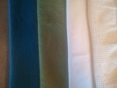
In a spirited act of geeky indulgence, I went to my linen closest, grabbed some tea towels, pulled out my phone (obviously), and captured this scene. A set of four folded tea towels overlapping and spread across my counter top—reverse engineering what I thought to be a suitable analogy for training my seismic inutition. The left (blue) tea towel is a honeycomb texture, the second (green) is speckled like a wash cloth, the third is a high thread-count linen, and the fourth has a grid of alternating cross-hatches and plain print. Don't laugh! It turns out to be quite difficult to verbally describe the patterns in these fabrics. Certainly, you will describe them differently to me, and that is the problem. 

Perhaps image processing can transcend our linguistic limitations. In seismic, as in image processing in general, there are attributes that work on each sample (or trace) independently, and there are attributes that use an ensemble of neighbouring samples in their computation. See if you can think a seismic analogy in the for each of these image attributes.

• Spectral decomposition shows the component of the RGB color spectrum at each sample location. I subsequently clipped and enhanced the red panel to show curves, wrinkles and boundaries caused by the interplay of light, shadows, and morphology.
• Spectral filtering extracts or removes hues. In this instance, I have selected all the color triplets that make up the blue tea towel. You could also select a range to say, show where the shadows are.
• Edge detection, after smoothing, shows sharp edges in white and yellow, soft edges in purple and blue. The wrinkles and subtle folds on the right most fabric have also been detected. 

My question: can you manually draw the morphology, or the blues, or the edges and discontinuities? Manual interpretation is time consuming, prone to error, seldom reproducible, and that makes it flawed. Furthermore, none of these attributes actually tell us about the nature of the textures in the fabric. Indeed, we don't know if any of them are relevant at all. Colour happens to be one proxy for texture in this case, but it fails in delineating the two whitish fabrics.

Artistically and computationally speaking, I submit to you that seismic data are nothing but images. In the next post I will extend this fabric-photograph model to explore the utility of textural attributes. 

Theses images were made using the open source FIJI and the illustrations were done in Inkscape. The attributes were computed in MATLAB and FIJI.

I is for integrated trace

A zero-phase wavelet has peaks and troughs that line up with interfaces, and has side-lobe events not associated with physical boundaries. Because of this, we see that seismic amplitude is only, at best, a proxy for earth's material contrasts (as shown below by the impedance log) and can be difficult to interpret. The largest positive amplitude corresponds to a downward increase in impedance, and the largest negative amplitude corresponds to a downward decrease in impedance.

Now consider the integral of the seismic trace. In the illustration, I have coloured the positive amplitude values blue, and the negative amplitude values red, for each time sample. The integral is literally the sample-by-sample cumulative sum of amplitudes. Notice how the shape of the trace integral now looks similar to the impedance log (far left). The inflections correlate to the bed boundaries; the integration has done a 90 degree phase rotation of the data. The integrated trace looks more like the geologic contrasts. To think of it another way, if the derivative of impedance is reflectivity, then the derivative of the integrated trace is the seismic trace.  

In the final column on the right, the integrated trace has been scaled so that the relative variations approximately match the absolute variations of the actual acoustic impedance log. This curve is merely a squeeze and bulkshift of the integrated trace, to align with the impedance of the background lithology. In practice, scaling seismic measurements to geologically realistic ranges requires the knowledge of rock properties from nearby well logs. The trace on the far right is a rudimentary geology-from-seismic transformation of the data. Although the general shape of the 3-layer model is reconstructed, there are some complications. The first and third layer is too soft, the middle layer is too hard (and wobbly). The appearance of a high impedance doublet is because the seismic is band-limited. 

It is important to note that a trace integral does not yield a seismic estimate of impedance, it is only a proxy. Consider it a starting point for seismic inversion, not a substitute for it. In oil sands, for instance, Matt showed how the integrated trace gives a considerably more robust estimate of impedance for reservoir characterization compared to a more time consuming and expensive seismic inversion process.

Integrated trace is not meant to be the final product in a reservoir characterization workflow, but it is a seismic attribute that you should be working with anytime you are are trying to do inversion. It should be a starting point, a sanity check, because it is fast to run, easy to understand, completely deterministic (no guess work). If it is not available on your standard interpretation software, Geocraft is one place where you can do it.

Randomness and thin beds

Day 2 of the SEG Annual Meeting brought another 93 talks in the morning, and 103 in the afternoon, leaving us bewildered again: how to choose ten or so talks to see? (We have some ideas on this, more of which another day). Matt tried just sitting through a single session (well, almost), whereas Evan adopted the migrant approach again. These are our picks, just for you.

Stewart Trickett, Kelman

There has never been a dull or difficult talk from Stewart, one of Calgary's smartest and most thoughtful programmer–processors. He has recently addressed the hot-topic of 5D interpolation, a powerful process for making the dream of cheap, dense sampling a reality. Today, he explained why we need to now think about optimizing acquisition not for imaging, but for interpolation. And interpolation really likes pseudorandom sampling, because it helps negotiate the terms & conditions of Nyquist and avoid spatial aliasing. He went on to show a 3D subsampled then imaged three ways: remove every other shot line, remove every other shot, or remove a random shot from every pair of shots. All reduce the fold to 12% of the full data. The result: pseudorandom sampling wins every time. But don't panic, the difference in the migrated images was much smaller than in the structure stacks.

Gaynor Payton, ffA

In what could have been a product-focused marketing talk, Gaynor did a good job of outlining five easy-to-follow, practical workflows for interpreters working on thin beds. She showed frequency- and phase-based methods that exploit near-tuning, unresolved doublets in the waveform. A nice-looking bandwidth enhancement result was followed up with ffA's new high-resolution spectral decomposition we covered recently. Then she showed how negative spikes in instantaneous frequency can reveal subtle doublets in the waveform. This was extended with a skeletonized image, a sort of band-limited reflectivity display. Finally, she showed an interesting display of signed trace slope, which seemed to reveal the extent of just-resolved doublets quite nicely.

Scott Mackay, consultant

Scott MacKay shared some of his deep experience with depth imaging, but specially translated for interpreters. And this is only right: depth imaging is first and foremost an interpretive, iterative process, not a product. He gave some basic heuristics, guiding principles for interpreters. The first velocity model should be smooth—really smooth. Iterations should be only incrementally less smooth, 'creeping up' on the solution. Structure should get less, not more, complex with each step. Gathers should be flattish, not flat. Be patient, and let the data speak. And above all, Don't Panic. Always good advice.

More posts about SEG 2011.

News of the week

The summer is, unbelievably, drawing in. While you've been gadding about in the sunshine, we've been scouring the geoscience and technology news — just for you! Here are some things that caught our eye in August. 

Spectral stuff from ffA

If you're a regular reader, you know we'll always cover a story about seismic frequency and resolution. A week ago, purveyors of high-tech seismic attributes ffA introduced HD Frequency Decomposition, or HDFD. As you might guess, HD stands for high definition, though it's not clear what that means in the context of seismic attributes. As is fairly normal with resolution-enhancing technology, the claims are eyebrow-raisingly bold:

...[we can] step beyond the resolution limitations of conventional frequency decomposition techniques.
Steve Purves, Technical Director, ffA

You can read about the technique in the nicely illustrated datasheet, but don't expect to find out how it works. I was disappointed to see that it doesn't even mention the type of decomposition; we assume it's some sort of scale-based approach (that is based on a wavelet, not Fourier, transform). Quiz them yourself at SEG next month in Booth C-1644.

By the way, if you're going to SEG and have a smart phone, think about keeping up with the buzz by following some chatterboxes on Twitter—@SEGAnnualMtg, @ParadigmLtd, @ESG_Solutions, @kwinkunks, and @EvanBianco. You can create and account and just follow the conversation, but it's more fun to join in!

More microseismic power for Canada

A good friend of Agile's recently went to work at Spectraseis, a seismic processing firm specializing in microseismic and reservoir monitoring in general. They just opened a Calgary office, so good luck to them in what is a pretty tight market (there must be 50 seismic processing shops in Calgary). The company also announced $3.6M of investment from Credit Suisse, so they are clearly on a roll.

Next gen knowledge management

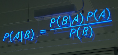
Repsol, the Spanish oil company and supercomputing powerhouse, is rolling out some new knowledge sharing technology from Autonomy, a fast-growing UK company. There are two pieces: IDOL, an enterprise search engine, and Virage, a rich media management system. 

Autonomy is an awesome company. How do we know this? They have Bayes' Theorem up in neon lights. Yeah, Bayes' Theorem. 

Get geo-referenced maps faster

Elsevier is one of the giants of 'old school' publishing, but also one of the more innovative ones (have you seen their graphical abstracts?). They have just introduced an awesome-looking search site for exploration geoscientists, called Geofacets. It's a set of power tools for finding maps and figures, already georeferenced and ready for a GIS. It even includes IHS's global basins map to search more geologically, and includes what you need to know about rights and permissions. If your company has ScienceDirect access, which they probably do, then you should have immediate access.

Previous news posts from Agile*

HD Frequency Decomposition is a trademark of ffA, IDOL and Virage are trademarks of Autonomy, Geofacets is a trademark of Elesevier. Bayes' Theorem image is CC-BY-SA licensed by its creator mattbuck. This regular news feature is for information only. We aren't connected with any of these organizations, and don't necessarily endorse their products or services.

How to cheat at spot the difference

Yesterday I left you, dear reader, with a spot the difference puzzle. Here it is again, with my answer:

Notice how my answer (made with GIMP) is not just a list of differences or a squiggly circle around each one. It's an exact map of the location and nature of every difference. I like the effect of seeing which 'direction' the difference goes in: blue things are in the left image but not the right. One flaw in this method is that I have reduced the image to a monochrome image; changes in colour only would not show up. 

Another way to do it, a way that would catch even a subtle colour change, is to simply difference the images. Let's look at a detail from the image—the yellow box; the difference is the centre image:

The right-hand image here is a further processing of the difference, using a process in ImageJ that inverts the pixels' values, making dark things bright and viceversa. This reveals a difference we would probably never have otherwise noticed: the footprint of the lossy JPEG compression kernel. Even though the two input images were compressed with 98% fidelity, we have introduced a subtle, but pervasive, artifact.

So what? Is this just an image processing gimmick? It depends how much you care about finding these differences. Not only was it easier to find all the differences this way, but now I know for certain that I have not missed any. We even see one or two very tiny differences that were surely unintentional (there's one just next to the cat's right paw). If differences (or similarities) mean a lot to you, because a medical prognosis or well location depends on their identification, the small ones might be very important!

View fullsize

Here's a small tutorial showing how I made the line difference, in case you are interested →

Visual crossplotting

To clarify, add detail
Edward Tufte

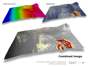
Pyroclastic flow on Nabro, Eritrea. Click for a larger image. NASA.Recently, the prolific geoblogger Brian Romans posted a pair of satellite images of a pyroclastic flow on Nabro in Eritrea. One image was in the visible spectrum, the other was a thermal image. Correlating them by looking back and forth at the images is unsatisying, so I spent 10 minutes merging the data into a single view, making the correlation immediate and intuitive. 

Maps like this are always better than abstractions of data like graphs or crossplots (or scatter plots, if you prefer). Plots get unwieldy with more than three dimensions, and there are almost always more dimensions to the data, especially in geoscience. In the image above there are at least half a dozen dimensions to the data: x and y position, elevation, slope, rugosity, vegetation (none!), heat intensity, heat distribution,... And these other dimensions, however tenuous or qualitative, might actually be important—they provide context, circumstantial evidence, if you will.

When I review papers, one of the comments I almost always make is: get all your data into one view—help your reader make the comparison. Instead of two maps showing slightly different seismic attributes, make one view and force the comparison. Be careful with colours: don't use them all up for one of the attributes, leaving nothing for the other. Using greys and blues for one leaves reds and yellows for the other. This approach is much more effective than a polygon around your anomaly, say, because then you have indelibly overlain your interpretation too early in the story: wait until you have unequivocally demonstrated the uncanny correlation.

If you're still not convinced that the richer image conveys more information, see how long it takes you to do this Spot The Difference. Come back tomorrow for the answer (and the point!)...

Creative Commons licensed image from Wikimedia Commons, work of User Muband (Japan)

GIMP is your friend!

Reliable predictions of unlikely geology

A puzzle

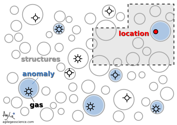
Imagine you are working in a newly-accessible and under-explored area of an otherwise mature basin. Statistics show that on average 10% of structures are filled with gas; the rest are dry. Fortunately, you have some seismic analysis technology that allows you to predict the presence of gas with 80% reliability. In other words, four out of five gas-filled structures test positive with the technique, and when it is applied to water-filled structures, it gives a negative result four times out of five.

← It is thought that 10% of the structures in this play are gas-filled. Your seismic attribute test is thought to be 80% reliable, because four out of five times it has indicated gas correctly. You acquire the undrilled acreage shown by the grey polygon.

You acquire some undrilled acreage—the grey polygon— then delineate some structures and perform the analysis. One of the structures tests positive. If this is the only information you have, what is the probability that it is gas-filled?

This is a classic problem of embracing Bayesian likelihood and ignoring your built-in 'representativeness heuristic' (Kahneman et al, 1982, Judgment Under Uncertainty: Heuristics and Biases, Cambridge University Press). Bayesian probability combination does not come very naturally to most people but, once understood, can at least help you see the way to approach similar problems in the future. The way the problem is framed here, it is identical to the original formulation of Kahneman et al, the Taxicab Problem. This takes place in a town with 90 yellow cabs and 10 blue ones. A taxi is involved in a hit-and-run, witnessed by a passer-by. Eye witness reliability is shown to be 80%, so if the witness says the taxi was blue, what is the probability that the cab was indeed blue? Most people go with 80%, but in fact the witness is probably wrong. To see why, let's go back to the exploration problem and look at 100 test cases.

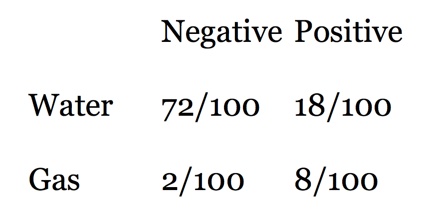
Break it down

Looking at the rows in this table of outcomes, we see that there are 90 water cases and 10 gas cases. Eighty percent of the water cases test negative, and 80% of the gas cases test positive. The table shows that when we get a positive test, the probability that the test is true is not 0.80, but much less: 8/(8+18) = 0.31. In other words, a test that is mostly reliable is probably wrong when applied to an event that doesn't happen very often (a structure being gas charged). It's still good news for us, though, because a probability of discovery of 0.31 is much better than the 0.10 that we started with.

Here is Bayes' Theorem for calculating the probability P of event A (say, a gas discovery) given event B (say, a positive test in our seismic analysis):

So we can express our problem in these terms:

Are you sure about that?

This result is so counter-intuitive, for me at least, that I can't resist illustrating it with another well-known example that takes it to extremes. Imagine you test positive for a very rare disease, seismitis. The test is 99% reliable. But the disease affects only 1 person in 10 000. What is the probability that you do indeed have seismitis?

Notice that the unreliability (1%) of the test is much greater than the rate of occurrence of the disease (0.01%). This is a red flag. It's not hard to see that there will be many false positives: only 1 person in 10 000 are ill, and that person tests positive 99% of the time (almost always). The problem is that 1% of the 9 999 healthy people, 100 people, will test positive too. So for every 10 000 people tested, 101 test positive even though only 1 is ill. So the probability of being ill, given a positive test, is only about 1/101!

Lessons learned

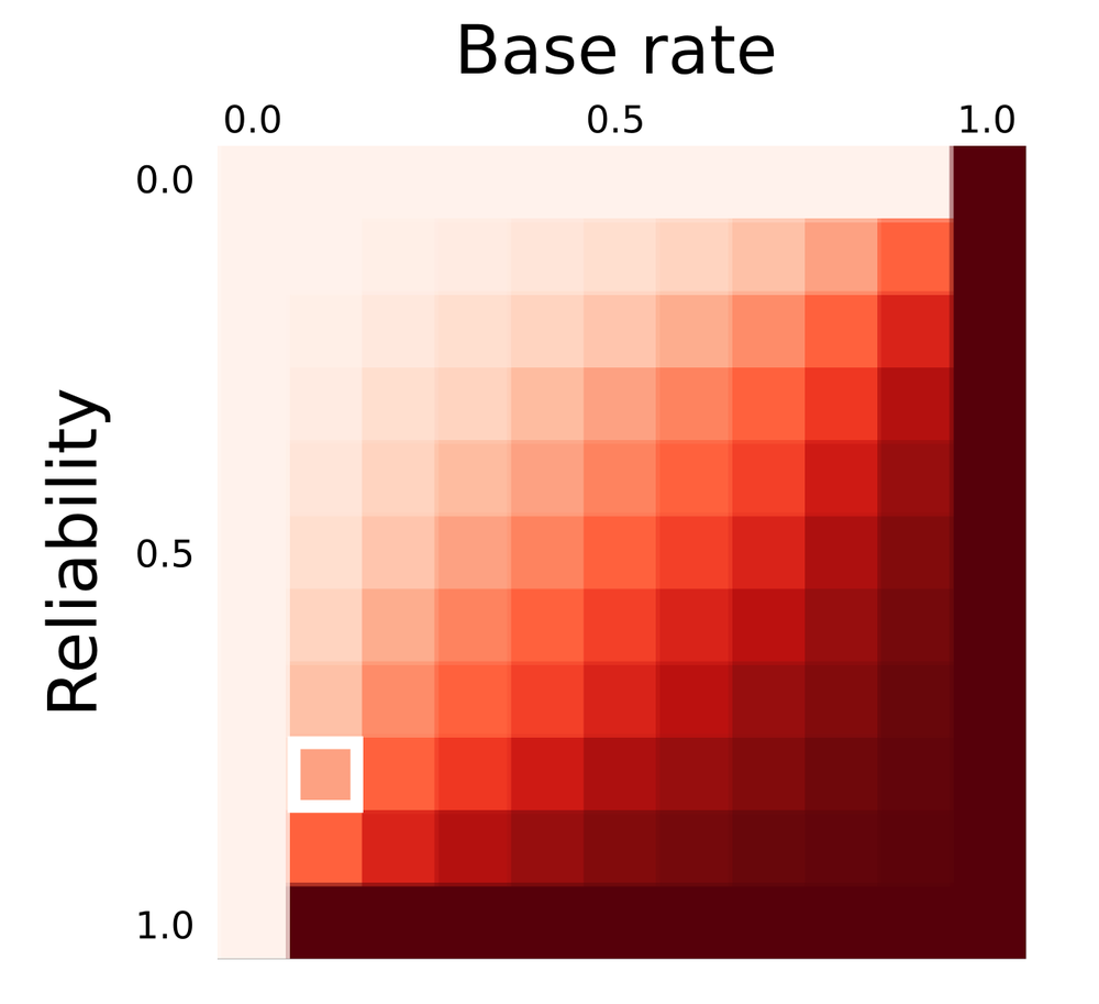
← Predictive power (in Bayesian jargon, the posterior probability) as a function of test reliability and the base rate of occurrence (also called the prior probability of the event of phenomenon in question). The position of the scenario in the exploration problem is shown by the white square.

Thanks to UBC Bioinformatics for the heatmap software, heatmap.notlong.com.

Next time you confidently predict something with a seismic attribute, stop to think not only about the reliability of the test you have made, but the rate of occurrence of the thing you're trying to predict. The heatmap shows how prediction power depends on both test reliability and the occurrence rate of the event. You may be doing worse (or better!) than you think.

Fortunately, in most real cases, there is a simple mitigation: use other, independent, methods of prediction. Mutually uncorrelated seismic attributes, well data, engineering test results, if applied diligently, can improve the odds of a correct prediction. But computing the posterior probability of event A given independent observations B, C, D, E, and F, is beyond the scope of this article (not to mention this author!).

This post is a version of part of my article The rational geoscientist, The Leading Edge, May 2010

Update on 2011-07-12 23:31 by Matt Hall

Just flicking through the archives and came across this post about unlikely events and Bayes' theorem. I can't believe I forgot to link to it in this story. So I'm doing it now!

E is for Envelope

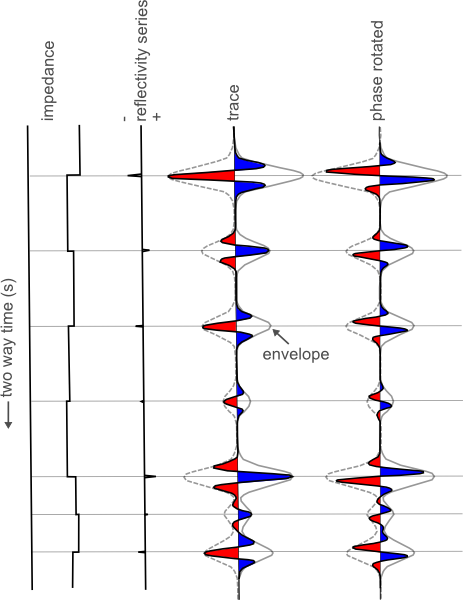
There are 8 layers in this simple blocky earth model. You might say that there are only 7 important pieces of information for this cartoon earth; the 7 reflectivity contrasts at the layer boundaries.

The seismic traces however, have more information than that. On the zero phase trace, there are 21 extrema (peaks / troughs). Worse yet, on the phase rotated trace there are 28. So somehow, the process of wave propagation has embedded more information than we need. Actually, in that case, maybe we shouldn't call it information: it's noise.

It can be hard to tell what is real and what is side lobe and soon, you are assigning geological significance to noise. A literal interpretation of the peaks and troughs would produce far more layers than there actually are. If you interpret every extreme as being matched with a boundary, you would be wrong.

Consider the envelope. The envelope has extrema positioned exactly at each boundary, and perhaps more importantly, it literally envelopes (I enunciate it differently here for drama) the part of the waveform associated with that reflection. 7 boundaries, 7 bumps on the envelope, correctly positioned in the time domain.

Notice how the envelope encompasses all phase rotations from 0 to 360 degrees; it's phase invariant. Does this make it more robust? But it's so broad! Are we losing precision or accuracy by accompanying our trace with it's envelope? What does vertical resolution really mean anyway?

Does this mean that every time there is an envelope maximum, I can expect a true layer boundary? I for one, don't know if this is fool proof in the face of interferring wavelets, but it has implications for how we work as seismic interpreters. Tomorrow we'll take a look at the envelope attribute in the context of real data.

Update on 2011-03-24 21:59 by Evan Bianco

Go to part two of this post to see how envelope can be applied to real data.