A stupid seismic model from core

On the plane back from Calgary, I got an itch to do some image processing on some photographs I took of the wonderful rocks on display at the core convention. Almost inadvertently, I composed a sequence of image filters that imitates a seismic response. And I came to these questions:  

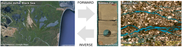
  • Is this a viable way to do forward modeling? 
  • Can we exploit scale invariance to make more accurate forward models?
  • Can we take the fabric from core and put it in a reservoir model?
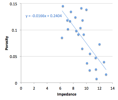
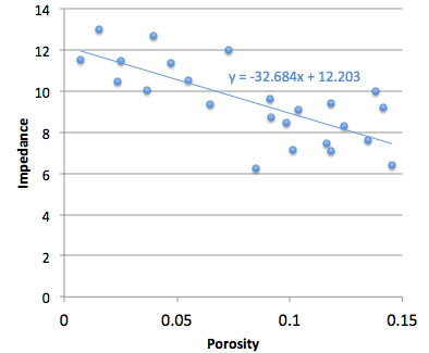
  • What is the goodness of fit between colour and impedance? 

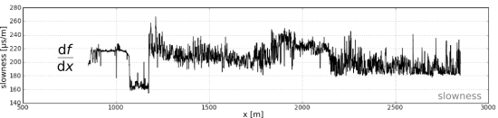
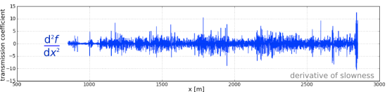
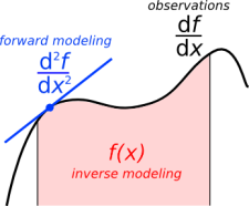
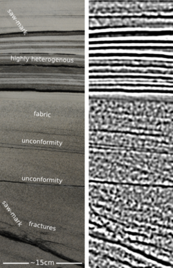
Click to enlargeAbove all, this image processing excerise shows an unambiguous demonstration of the effects of bandwidth. The most important point, no noise has been added. Here is the sequence, it is three steps: convert to grayscale, compute Laplacian, apply bandpass filter. This is analgous to the convolution of a seismic wavelet and the earth's reflectivity. Strictly speaking, it would be more physically sound to make a forward model using wavelet convolution (simple) or finite difference simulation (less simple), but that level of rigour was beyond the scope of my tinkering.

The two panels help illustrate a few points. First, finely layered heterogeneous stratal packages coalesce into crude seismic events. This is the effect of reducing bandwidth. Second, we can probably argue about what is 'signal' and what is 'noise'. However, there is no noise, per se, just geology that looks noisy. What may be mistaken as noise, might in fact be bonafide interfaces within material properties. 

If the geometry of geology is largely scale invariant, perhaps, just perhaps, images like these can be used at the basin and reservoir scale. I really like the look of the crumbly fractures near the bottom of the image. This type of feature could drive the placement of a borehole, and the production in a well. The patches, speckles, and bands in the image are genuine features of the geology, not issues of quality or noise. 

Do you think there is a role for transforming photographs of rocks into seismic objects?

Fitting a model to data

In studying the earth, we can't afford to take enough observations, and they will never be free of noise. So if you say you do geoscience, I hereby challenge you to formulate your work as a mathematical inverse problem. Inversion is a question: given the data, the physical equations, and details of the experiment, what is the distribution of physical properties? To answer this question we must address three more fundamental ones (Scales, Smith, and Treitel, 2001):

  • How accurate is the data? Or what does fit mean?
  • How accurately can we model the response of the system? Have we included all the physics that can contribute signifcantly to the data?
  • What is known about the system independent of the data? There must be a systematic procedure for rejecting unreasonable models that fit the data as well.

Setting up an inverse problem means coming up with the equations that contain the physics and geometry of the system under study. The method for solving it depends on the nature of the system of equations. The simplest is the minimum norm solution, and you've heard of it before, but perhaps under a different name.

To fit is to optimize a system of equations

For problems where the number of observations is greater than the number of unknowns, we want to find which unknowns fit the best. One case you're already familiar with is the method of least squares — you've used it fitting a line of through a set of points. A line is unambiguously described by only two parameters: slope a and y-axis intercept b. These are the unknowns in the problem, they are the model m that we wish to solve for. The problem of line-fitting through a set of points can be written out like this,

As I described in a previous post, the system of the problem takes the form d = Gm, where each row links a data point to an equation of a line. The model vector m (M × 1), is smaller than the data d (N × 1) which makes it an over-determined problem, and G is a N × M matrix holding the equations of the system.

Why cast a system of equations in this matrix form? Well, it turns out that the the best-fit line is precisely,

which are trivial matrix operations, once you've written out G.  T means to take the transpose, and –1 means the inverse, the rest is matrix multiplication. Another name for this is the minimum norm solution, because it defines the model parameters (slope and intercept) for which the lengths (vector norm) between the data and the model are a minimum. 

One benefit that comes from estimating a best-fit model is that you get the goodness-of-fit for free. Which is convenient because making sense of the earth doesn't just mean coming up with models, but also expressing their uncertainty, in terms of the errors with which they are linked.

I submit to you that every problem in geology can be formulated as a mathematical inverse problem. The benefit of doing so is not just to do math for math's sake, but it is only through quantitatively portraying ambiguous inferences and parameterizing non-uniqueness that we can do better than interpreting or guessing. 

Reference (well worth reading!)

Scales, JA, Smith, ML, and Treitel, S (2001). Introductory Geophysical Inverse Theory. Golden, Colorado: Samizdat Press

Backwards and forwards reasoning

Most people, if you describe a train of events to them will tell you what the result will be. There will be few people however, that if you told them a result, would be able to evolve from their own consciousness what the steps were that led to that result. This is what I mean when I talk about reasoning backward.

— Sherlock Holmes, A Study in Scarlet, Sir Arthur Conan Doyle (1887)

Reasoning backwards is the process of solving an inverse problem — estimating a physical system from indirect data. Straight-up reasoning, which we call the forward problem, is a kind of data collection: empiricism. It obeys a natural causality by which we relate model parameters to the data that we observe.

Modeling a measurement

Marmousi_Forward_Inverse_800px.png

Where are you headed? Every subsurface problem can be expressed as the arrow between two or more such panels.Inverse problems exists for two reasons. We are incapable of measuring what we are actually interested in, and it is impossible to measure a subject in enough detail, and in all aspects that matter. If, for instance, I ask you to determine my weight, you will be troubled if the only tool I allow is a ruler. Even if you are incredibly accurate with your tool, at best, you can construct only an estimation of the desired quantity. This estimation of reality is what we call a model. The process of estimation is called inversion.

Measuring a model

Forward problems are ways in which we acquire information about natural phenomena. Given a model (me, say), it is easy to measure some property (my height, say) accurately and precisely. But given my height as the starting point, it is impossible to estimate the me from which it came. This is an example of an ill-posed problem. In this case, there is an infinite number of models that share my measurements, though each model is described by one exact solution. 

Solving forward problems are nessecary to determine if a model fits a set of observations. So you'd expect it to be performed as a routine compliment to interpretation; a way to validate our assumptions, and train our intuition.  

The math of reasoning

Forward and inverse problems can be cast in this seemingly simple equation.

Gm=d

where d is a vector containing N observations (the data), m is a vector of M model parameters (the model), and G is a N × M matrix operator that connects the two. The structure of G changes depending on the problem, but it is where 'the experiment' goes. Given a set of model parameters m, the forward problem is to predict the data d produced by the experiment. This is as simple as plugging values into a system of equations. The inverse problem is much more difficult: given a set of observations d, estimate the model parameters m.

Marmousi_G_Model_Data_800px_updated.png

I think interpreters should describe their work within the Gm = d framework. Doing so would safeguard against mixing up observations, which should be objective, and interpretations, which contain assumptions. Know the difference between m and d. Express it with an arrow on a diagram if you like, to make it clear which direction you are heading in.

Illustrations for this post were created using data from the Marmousi synthetic seismic data set. The blue seismic trace and its corresponding velocity profile is at location no. 250.

How to get paid big bucks

Yesterday I asked 'What is inversion?' and started looking at problems in geoscience as either forward problems or inverse problems. So what are some examples of inverse problems in geoscience? Reversing our forward problem examples:

  • Given a suite of sedimentological observations, provide the depositional environment. This is a hard problem, because different environments can produce similar-looking facies. It is ill-conditioned, because small changes in the input (e.g. the presence of glaucony, or Cylindrichnus) produces large changes in the interpretation.
  • Given a seismic trace, produce an impedance log. Without a wavelet, we cannot uniquely deduce the impedance log — there are infinitely many combinations of log and wavelet that will give rise to the same seismic trace. This is the challenge of seismic inversion. 

To solve these problems, we must use induction — a fancy name for informed guesswork. For example, we can use judgement about likely wavelets, or the expected geology, to constrain the geophysical problem and reduce the number of possibilities. This, as they say, is why we're paid the big bucks. Indeed, perhaps we can generalize: people who are paid big bucks are solving inverse problems...

  • How do we balance the budget?
  • What combination of chemicals might cure pancreatic cancer?
  • What musical score would best complement this screenplay?
  • How do I act to portray a grief-stricken war veteran who loves ballet?

What was the last inverse problem you solved?

What is inversion?

Inverse problems are at the heart of geoscience. But I only hear hardcore geophysicists talk about them. Maybe this is because they're hard problems to solve, requiring mathematical rigour and computational clout. But the language is useful, and the realization that some problems are just damn hard — unsolvable, even — is actually kind of liberating. 

Forwards first

Before worrying about inverse problems, it helps to understand what a forward problem is. A forward problem starts with plenty of inputs, and asks for a straightforward, algorithmic, computable output. For example:

  • What is 4 × 5?
  • Given a depositional environment, what sedimentological features do we expect?
  • Given an impedance log and a wavelet, compute a synthetic seismogram.

These problems are solved by deductive reasoning, and have outcomes that are no less certain than the inputs.

Can you do it backwards?

You can guess what an inverse problem looks like. Computing 4 × 5 was pretty easy, even for a geophysicist, but it's not only difficult to do it backwards, it's impossible:

20 = what × what

You can solve it easily enough, but solutions are, to use the jargon, non-unique: 2 × 10, 7.2 × 1.666..., 6.3662 × π — you get the idea. One way to deal with such under-determined systems of equations is to know about, or guess, some constraints. For example, perhaps our system — our model — only includes integers. That narrows it down to three solutions. If we also know that the integers are less than 10, there can be only one solution.

Non-uniqueness is a characteristic of ill-posed problems. Ill-posedness is a dead giveaway of an inverse problem. Proposed by Jacques Hadamard, the concept is the opposite of well-posedness, which has three criteria:

  • A solution exists.
  • The solution is unique.
  • The solution is well-conditioned, which means it doesn't change disproportionately when the input changes. 

Notice the way the example problem was presented: one equation, two unknowns. There is already a priori knowledge about the system: there are two numbers, and the operator is multiplication. In geoscience, since the earth is not a computer, we depend on such knowledge about the nature of the system — what the variables are, how they interact, etc. We are always working with a model of nature.

Tomorrow, I'll look at some specific examples of inverse problems, and Evan will continue the conversation next week.

The calculus of geology

Calculus is the tool for studying things that change. Even so, in the midst of the dynamic and heterogeneous earth, calculus is an under-practised and, around the water-cooler at least, under-celebrated workhorse. Maybe that's because people don't realize it's all around us. Let's change that. 

Derivatives of duration

We can plot the time f(x) that passes as a seismic wave travels though space x. This function is known to many geophysicists as the time-to-depth function. It is key for converting borehole measurements, effectively recorded using a measuring tape, to seismic measurements, recorded using a stop watch.

Now let's take the derivative of f(x) with repsect to x. The result is the slowness function (the reciprocal of interval velocity):

The time duration that a seismic wave travels over a small interval (one metre). This function is an actual sonic well log. Differentiating once again yields this curious spiky function:

Geophysicists will spot that this resembles a reflection coefficient series, which governs seismic amplitudes. This is actually a transmission coefficient function, but that small detail is beside the point. In this example, the creating a synthetic seismogram mimics the calculus of geology. 

If you are familiar with the integrated trace attribute, you will recognize that it is an attempt to compute geology by integrating reflectivity spikes. The only issue in this case, and it is a major issue, is that the seismic trace is bandlimited. It does not contain all the information about the earth's slowness. So the earth's geology remains elusive and blurry.

The derivative of slowness yields the reflection boundaries, the integral of slowness yields their position. So in geophysics speak, I wonder, is forward modeling akin to differentiation, and inverse modeling akin to integration? I find it fascinating that these three functions have essentially the same density of information, yet they look increasingly complicated when we take derivatives. 

What other functions do you come across that might benefit from the calculus treatment?

The sonic log used in this example is from the O-32-B/11-E-64 well onshore Nova Scotia, which is publically available but not easily accessible online.

Ten ways to spot pseudogeophysics

Geophysicists often try to predict rock properties using seismic attributes — an inverse problem. It is difficult and can be complicated. It can seem like black magic, or at least a black box. They can pull the wool over their own eyes in the process, so don’t be surprised if it seems like they are trying to pull the wool over yours. Instead, ask a lot of questions.

Questions to ask

  1. What is the reliability of the logs that are inputs to the prediction? Ask about hole quality and log editing.
  2. What about the the seismic data? Ask about signal:noise, multiples, bandwidth, resolution limits, polarity, maximum offset angle (for AVO studies), and processing flow (e.g. Emsley, 2012).
  3. What is the quality of the well ties? Is the correlation good enough for the proposed application?
  4. Is there any physical reason why the seismic attribute should predict the proposed rock property? Was this explained to you? Were you convinced?
  5. Is the proposed attribute redundant (sensu Barnes, 2007)? Does it really give better results than a less sexy approach? I’ve seen 5-minute trace integration outperform month-long AVO inversions (Hall et al. 2006).
  6. What are the caveats and uncertainties in the analysis? Is there a quantitative, preferably Bayesian, treatment of the reliability of the predictions being made? Ask about the probability of a prediction being wrong.
  7. Is there a convincing relationship between the rock property (shear impedance, say) and some geologically interesting characteristic that you actually make decisions with, e.g. frackability.
  8. Is there a convincing relationship between the rock property and the seismic attribute at the wells? In other words, does the attribute actually correlate with the property where we have data?
  9. What does the low-frequency model look like? How was it made? Its maximum frequency should be about the same as the seismic data's minimum, no more.
  10. Does the geophysicist compute errors from the training error or the validation error? Training errors are not helpful because they beg the question by comparing the input training data to the result you get when you use those very data in the model. Funnily enough, most geophysicists like to show the training error (right), but if the model is over-fit then of course it will predict very nicely at the well! But it's the reliability away from the wells we are interested in, so we should examine the error we get when we pretend the well isn't there. I prefer this to witholding 'blind' wells from the modeling — you should use all the data. 

Lastly, it might seem harsh but we could also ask if the geophysicist has a direct financial interest in convincing you that their attribute is sound, as well as the normal direct professional interest. It’s not a problem if they do, but be on your guard — people who are selling things are especially prone to bias. It's unavoidable.

What do you think? Are you bamboozled by the way geophysicists describe their predictions?

References
Barnes, A (2007). Redundant and useless seismic attributes. Geophysics 72 (3), p P33–P38. DOI: 10.1190/1.2370420.
Emsley, D. Know your processing flow. In: Hall & Bianco, eds, 52 Things You Should Know About Geophysics. Agile Libre, 2012. 
Hall, M, B Roy, and P Anno (2006). Assessing the success of pre-stack inversion in a heavy oil reservoir: Lower Cretaceous McMurray Formation at Surmont. Canadian Society of Exploration Geophysicists National Convention, Calgary, Canada, May 2006. 

The image of the training error plot — showing predicted logs in red against input logs — is from Hampson–Russell's excellent EMERGE software. I'm claiming the use of the copyrighted image is fair use.  

L is for Lambda

Hooke's law says that the force F exerted by a spring depends only on its displacement x from equilibrium, and the spring constant k of the spring:

.

We can think of k—and experience it—as stiffness. The spring constant is a property of the spring. In a sense, it is the spring. Rocks are like springs, in that they have some elasticity. We'd like to know the spring constant of our rocks, because it can help us predict useful things like porosity. 

Hooke's law is the basis for elasticity theory, in which we express the law as

stress [force per unit area] is equal to strain [deformation] times a constant

This time the constant of proportionality is called the elastic modulus. And there isn't just one of them. Why more complicated? Well, rocks are like springs, but they are three dimensional.

In three dimensions, assuming isotropy, the shear modulus μ plays the role of the spring constant for shear waves. But for compressional waves we need λ+2μ, a quantity called the P-wave modulus. So λ is one part of the term that tells us how rocks get squished by P-waves.

These mysterious quantities λ and µ are Lamé's first and second parameters. They are intrinsic properties of all materials, including rocks. Like all elastic moduli, they have units of force per unit area, or pascals [Pa].

So what is λ?

Matt and I have spent several hours discussing how to describe lambda. Unlike Young's modulus E, or Poisson's ratio ν, our friend λ does not have a simple physical description. Young's modulus just determines how much longer something gets when I stretch it. Poisson's ratio tells how much fatter something gets if I squeeze it. But lambda... what is lambda?

  • λ is sometimes called incompressibility, a name best avoided because it's sometimes also used for the bulk modulus, K.  
  • If we apply stress σ1 along the 1 direction to this linearly elastic isotropic cube (right), then λ represents the 'spring constant' that scales the strain ε along the directions perpendicular to the applied stress.
  • The derivation of Hooke's law in 3D requires tensors, which we're not getting into here. The point is that λ and μ help give the simplest form of the equations (right, shown for one dimension).

The significance of elastic properties is that they determine how a material is temporarily deformed by a passing seismic wave. Shear waves propagate by orthogonal displacements relative to the propagation direction—this deformation is determined by µ. In contrast, P-waves propagate by displacements parallel to the propagation direction, and this deformation is inversely proportional to M, which is 2µ + λ

Lambda rears its head in seismic petrophysics, AVO inversion, and is the first letter in the acronym of Bill Goodway's popular LMR inversion method (Goodway, 2001). Even though it is fundamental to seismic, there's no doubt that λ is not intuitively understood by most geoscientists. Have you ever tried to explain lambda to someone? What description of λ do you find useful? I'm open to suggestions. 

Goodway, B., 2001, AVO and Lame' constants for rock parameterization and fluid detection: CSEG Recorder, 26, no. 6, 39-60.

Cross plots: a non-answer

On Monday I asked whether we should make crossplots according to statistical rules or natural rules. There was some fun discussion, and some awesome computation from Henry Herrera, and a couple of gems:

Physics likes math, but math doesn't care about physics — @jeffersonite

But... when I consider the intercept point I cannot possibly imagine a rock that has high porosity and zero impedance — Matteo Niccoli, aka @My_Carta

I tried asking on Stack Overflow once, but didn’t really get to the bottom of it, or perhaps I just wasn't convinced. The consensus seems to be that the statistical answer is to put porosity on y-axis, because that way you minimize the prediction error on porosity. But I feel—and this is just my flaky intuition talking—like this fails to represent nature (whatever that means) and so maybe that error reduction is spurious somehow.

Reversing the plot to what I think of as the natural, causation-respecting plot may not be that unreasonable. It's effectively the same as reducing the error on what was x (that is, impedance), instead of y. Since impedance is our measured data, we could say this regression respects the measured data more than the statistical, non-causation-respecting plot.

So must we choose? Minimize the error on the prediction, or minimize the error on the predictor. Let's see. In the plot on the right, I used the two methods to predict porosity at the red points from the blue. That is, I did the regression on the blue points; the red points are my blind data (new wells, perhaps). Surprisingly, the statistical method gives an RMS error of 0.034, the natural method 0.023. So my intuition is vindicated! 

Unfortunately if I reverse the datasets and instead model the red points, then predict the blue, the effect is also reversed: the statistical method does better with 0.029 instead of 0.034. So my intuition is wounded once more, and limps off for an early bath.

Irreducible error?

Here's what I think: there's an irreducible error of prediction. We can beg, borrow or steal error from one variable, but then it goes on the other. It's reminiscent of Heisenberg's uncertainty principle, but in this case, we can't have arbitrarily precise forecasts from imperfectly correlated data. So what can we do? Pick a method, justify it to yourself, test your assumptions, and then be consistent. And report your errors at every step. 

I'm reminded of the adage 'Correlation does not equal causation.' Indeed. And, to borrow @jeffersonite's phrase, it seems correlation also does not care about causation.

Cross plot or plot cross?

I am stumped. About once a year, for the last nine years or so, I have failed to figure this out.

What could be simpler than predicting porosity from acoustic impedance? Well, lots of things, but let’s pretend for a minute that it’s easy. Here’s what you do:

1.   Measure impedance at a bunch of wells
2.   Measure the porosity — at seismic scale of course — at those wells
3.   Make a crossplot with porosity on the y-axis and amplitude on the x-axis
4.   Plot the data points and plot the regression line (let’s keep it linear)
5.   Find the equation of the line, which is of the form y = ax + b, or porosity = gradient × impedance + constant
6.   Apply the equation to a map (or volume, if you like) of amplitude, and Bob's your uncle.

Easy!

But, wait a minute. Is Bob your uncle after all? The parameter on the y-axis is also called the dependent variable, and that on the x-axis the independent. In other words, the crossplot represents a relationship of dependency, or causation. Well, porosity certainly does not depend on impedance — it’s the other way around. To put it another way, impedance is not the cause of porosity. So the natural relationship should put impedance, not porosity, on the y-axis. Right?

Therefore we should change some steps:

3.   Make a crossplot with impedance on the y-axis and porosity on the x-axis
4.   Plot the data points and plot the regression line
5a. Find the equation of the line, which is of the form y = ax + b, or impedance = gradient × porosity + constant
5b. Rearrange the equation for what we really want:
porosity = (impedance – constant)/gradient

Not quite as easy! But still easy.

More importantly, this gives a different answer. Bob is not your uncle after all. Bob is your aunt. To be clear: you will compute different porosities with these two approaches. So then we have to ask: which is correct? Or rather, since neither going to give us the ‘correct’ porosity, which is better? Which is more physical? Do we care about physicality?

I genuinely do not know the answer to this question. Do you?

If you're interested in playing with this problem, the data I used are from Imaging reservoir quality seismic signatures of geologic effects, report number DE-FC26-04NT15506 for the US Department of Energy by Gary Mavko et al. at Stanford University. I digitized their figure D-8; you can download the data as a CSV here. I have only plotted half of the data points, so I can use the rest as a blind test.