100 years of seismic reflection

Where would we be without seismic reflection? Is there a remote sensing technology that is as unlikely, as difficult, or as magical as the seismic reflection method? OK, maybe neutrino tomography. But anyway, seismic has contributed a great deal to society — helping us discover and describe hydrocarbon resources, aquifers, geothermal anomalies, sea-floor hazards, and plenty more besides.

It even indirectly led to the integrated circuit, but that’s another story.

Depending on who you ask, 9 August 2021 may or may not be the 100th anniversary of the seismic reflection method. Or maybe 5th August. Or maybe it was June or July. But there’s no doubt that, although the first discovery with seismic did not happen until several years later, 1921 was the year that the seismic reflection method was invented.

Ryan, Karcher and Haseman in the field, August 1921. Badly colourized by an AI.

Ryan, Karcher and Haseman in the field, August 1921. Badly colourized by an AI.

The timeline

I’ve tried to put together a timeline by scouring a few sources. Several people — Clarence Karcher (a physicist), William Haseman (a physicist), Irving Perrine (a geologist), William Kite (a geologist) at the University of Oklahoma, and later Daniel Ohern (a geologist) — conducted the following experiments:

  • 12 April 1919 — Karcher recorded the first exploration seismograph record near the National Bureau of Standards (now NIST) in Washington, DC.

  • 1919 to 1920 — Karcher continues his experimentation.

  • April 1921 — Karcher, whilst working at the National Bureau of Standards in Washington, DC, designed and constructed apparatus for recording seismic reflections.

  • 4 June 1921 — the first field tests of the refleciton seismograph at Belle Isle, Oklahoma City, using a dynamite source.

  • 6 June until early July — various profiles were acquired at different offsets and spacings.

  • 14 July 1921 — Testing in the Arbuckle Mountains. The team of Karcher, Haseman, Ohern and Perrine determined the velocities of the Hunton limestone, Sylvan shale, and Viola limestone.

  • Early August 1921 — The group moves to Vines Branch where “the world’s first reflection seismograph geologic section was measured”, according to a commemorative plaque on I-35 in Oklahoma. That plaque claims it was 9 August, but there are also records from 5 August. The depth to the Viola limestone is recorded and observed to change with geological structure.

  • 1 September 1921 — Karcher, Haseman, and Rex Ryan (a geologist) conduct experiments at the Newkirk Anticline near Ponca City.

  • 13 September 1921 — a survey was begun for Marland Oil Company and continues into October. Success seems mixed.

So what did these physicists and geologists actually do? Here’s an explanation from Bill Dragoset in his excellent review of the history of seismic from 2005:

Using a dynamite charge as a seismic source and a special instrument called a seismograph, the team recorded seismic waves that had traveled through the subsurface of the earth. Analysis of the recorded data showed that seismic reflections from a boundary between two underground rock layers had been detected. Further analysis of the data produced an image of the subsurface—called a seismic reflection profile—that agreed with a known geologic feature. That result is widely regarded as the first proof that an accurate image of the earth’s subsurface could be made using reflected seismic waves.
— Bill Dragoset, A Historical Reflection on Reflections

The data was a bit hard to interpret! This is from William Schriever’s paper:

Marland_seismic.png

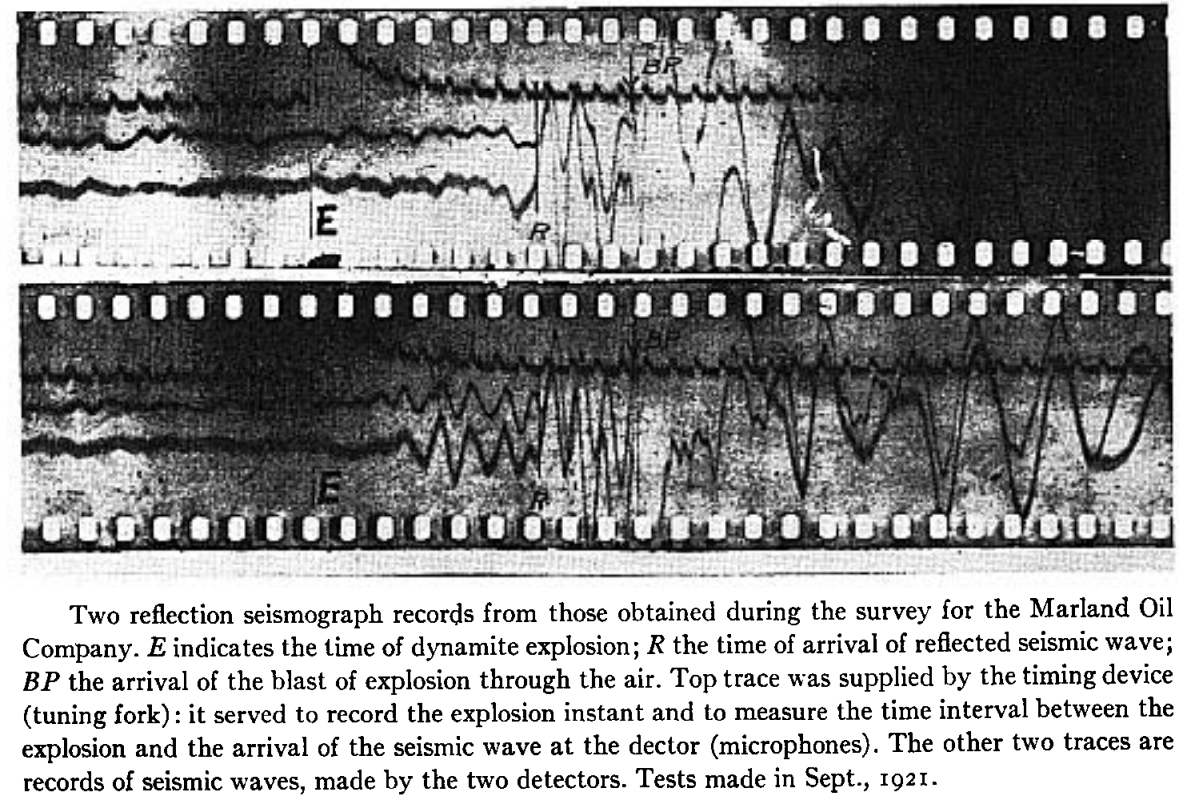
Nonetheless, here’s the section the team managed to draw at Vine Creek. This is the world’s first reflection seismograph section — 9 August 1921:

The method took a few years to catch on — and at least a few years to be credited with a discovery. Karcher founded Geophysical Research Corporation (now Sercel) in 1925, then left and founded Geophysical Service International — which later spun out Texas Instruments — in 1930. And, eventually, seismic reflection turned into an idsutry worth tens of billions of dollars per year. Sometimes.

References

Bill Dragoset, (2005), A historical reflection on reflections, The Leading Edge 24: s46-s70. https://doi.org/10.1190/1.2112392

Clarence Karcher (1932). DETERMINATION OF .SUBSURFACE FORMATIONS. Patent no. 1843725A. Patented 2 Feb 1932.

William Schriever (1952). Reflection seismograph prospecting; how it started; contributions. Geophysics 17 (4): 936–942. doi: https://doi.org/10.1190/1.1437831

B Wells and K Wells (2013). American Oil & Gas Historical Society. American Oil & Gas Historical Society. Exploring Seismic Waves. Last Updated: August 7, 2021. Original Published Date: April 29, 2013.

A forensic audit of seismic data

The SEG-Y “standard” is famously non-standard. (Those air quotes are actually part of the “standard”.)

For example, the inline and crossline location of a given trace — two things that you must have in order to load the data vaguely properly — are “recommended” (remember, it’s a “standard”) to be given in the trace’s header, at byte locations 189 and 193 respectively. Indeed, they might well be there. Or 1 and 5 (well, 5 or 9). Or somewhere else. Or not there at all.

Don Robinson at Resolve told me recently that he has seen more than 180 byte-location combinations, and he said another service company had seen more than 300.

All this can make loading seismic data really, really annoying.

I’d like to propose that the community performs a kind of forensic audit of SEG-Y files. I have 5 main questions:

  1. What proportion of files claim to be Rev 0, Rev 1, and Rev 2? And what standard are they actually? (If any!)

  2. What proportion of files in the wild use IBM vs IEEE floats? What about integers?

  3. What proportion of files in the wild use little-endian vs big-endian byte order. (Please tell me there's no middle-endian data out there!)

  4. What proportion of files in the wild use EBCDIC vs ASCII encoded textual file headers? (Again, I would hope there are no other encodings in use, but I bet there are.)

  5. What proportion of files use the Strongly recommended and Recommended byte locations for trace numbers, sample counts, sample interval, coordinates and inline–crossline numbers?

For each of these <things> it would also be interesting to know:

  • How does <thing> vary with the other things? That is, what's the cross-correlation matrix?

  • How does <thing> vary with the age of the file? Is there a temporal trend?

  • How does <thing> vary with the provenance of the file? What's the geographic trend? (For example, Don told me that the prevalence of PC-based interpretation packages in Canada led to widespread early adoption of IEEE floats and little-endian byte order; indeed, he says that 90% of the SEG-Y he sees in the wild is still IBM ormatted floats!)

While we’re at it, I'd also like in some more esoteric things:

  • How many files have cornerpoints in the text header, and/or trace locations in trace headers?

  • How many files have an unambiguous CRS in the text header?

  • How many files have information about the processing sequence in the text header? (E.g. imaging details, filters, etc.)

  • How many files have incorrect information in the headers (e.g. locations, sample interval, byte format, etc)

  • How many processors bother putting useful things like elevation, filters, sweeps, fold at target, etc, in the trace headers?

I don’t quite know how such a survey would happen. Most of these things are obviously detectable from the files themselves. Perhaps some of the many seismic data management systems already track these things. Or maybe you’re a data manager and you have some anecdotal data you can share.

What do you think? I’d love to hear your thoughts in the comments. Maybe there’s a good hackathon project here!

All the wedges

Wedges are a staple of the seismic interpreter’s diet. These simple little models show at a glance how two seismic reflections interact with each other when a rock layer thins down to — and below — the resolution limit of the data. We can also easily study how the interaction changes as we vary the wavelet’s properties, especially its frequency content.

Here’s how to make and plot a basic wedge model with Python in the latest version of bruges, v0.4.2:

 
import bruges as bg
import matplotlib.pyplot as plt

wedge, *_ = bg.models.wedge()

plt.imshow(wedge)
wedge_basic.png

It really is that simple! This model is rather simplistic though: it contains no stratigraphy, and the numerical content of the 2D array is just a bunch of integers. Let’s instead make a P-wave velocity model, with an internal bed of faster rock inside the wedge:

 
strat = [2.35, (2.40, 2.50, 2.40), 2.65]
wedge, *_ = bg.models.wedge(strat=strat)

plt.imshow(wedge)
plt.colorbar()
wedge_layer.png

We can also choose to make the internal geometry top- or bottom-conformant, mimicking onlap or an unconformity, respectively.

 
strat = strat=[0, 7*[1,2], 3]
wedge, *_ = bg.models.wedge(strat=strat,
                            conformance='base'
                           )

plt.imshow(wedge)
wedge_unconformity.png

The killer feature of this new function might be using a log to make the stratigraphy, rather than just a few beds. This is straightforward to do with welly, because it makes selecting depth intervals and resampling a bit easier:

 
import welly

gr = welly.Well.from_las('R-39.las').data['GR']
log_above = gr.to_basis(stop=2620, step=1.0)
log_wedge = gr.to_basis(start=2620, stop=2720, step=1.0)
log_below = gr.to_basis(start=2720, step=1.0)

strat = (log_above, log_wedge, log_below)
depth, width = (100, 400, 100), (40, 200, 40)
wedge, top, base, ref = bg.models.wedge(depth=depth,
                                        width=width,
                                        strat=strat,
                                        thickness=(0, 1.5)
                                       )

plt.figure(figsize=(15, 6))
plt.imshow(wedge, aspect='auto')
plt.axvline(ref, color='k', ls='--')
plt.plot(top, 'r', lw=2)
plt.plot(base, 'r', lw=2)
wedge_log.png

Notice that the function returns to you the top and base of the wedgy part, as well as the position of the ‘reference’, in this case the well.

I’m not sure if anyone wanted this feature… but you can make clinoform models too:

wedge_log_clino.png

Lastly, the whole point of all this was to make a synthetic — the forward model of the seismic experiment. We can make a convolutional model with just a few more lines of code:

 
strat = np.array([2.32 * 2.65,  # Layer 1
                  2.35 * 2.60,  # Layer 2
                  2.35 * 2.62,  # Layer 3
                 ])

# Fancy indexing into the rocks with the model.
wedge, top, base, ref = bg.models.wedge(strat=strat)

# Make reflectivity.
rc = (wedge[1:] - wedge[:-1]) / (wedge[1:] + wedge[:-1])

# Get a wavelet.
ricker = bg.filters.ricker(0.064, 0.001, 40)

# Repeated 1D convolution for a synthetic.
syn = np.apply_along_axis(np.convolve, arr=rc, axis=0, v=ricker, mode='same')
wedge_synthetic.png

That covers most of what the tool can do — for now. I’m working on extending the models to three dimensions, so you will be able to vary layers or rock properties in the 3rd dimension. In the meantime, take these wedges for a spin and see what you can make! Do share your models on Twitter or LinkedIn, and have fun!

x lines of Python: static basemaps with contextily

Difficulty rating: Beginner

Something that is often useful in planning is to have a basemap of the area in which you have data or an interest. This can be made using a number of different tools, up to and including full-fledged GIS software, but we will use Contextily for a quick static basemap using Python. Installation is as simple as using conda install contextily or pip install contextily.

The steps that we want to take are the following, expressed in plain English, each of which will roughly be one line of code:

  1. Get a source for our basemap (placenames and similar things)
  2. Get a source for our geological map
  3. Get the location that we would like to map
  4. Plot the location with our geological data
  5. Add the basemap to our geological map
  6. Add the attribution for both maps
  7. Plot our final map

We will start with the imports, which as usual do not count:

 
import contextily as ctx
import matplotlib.pyplot as plt

Contextily has a number of built-in providers of map tiles, which can be accessed using the ctx.providers dictionary. This is nested, with some providers offering multiple tiles. An example is the ctx.providers.OpenStreetMap.Mapnik provider, which contains the following:

 
{'url': 'https://{s}.tile.openstreetmap.org/{z}/{x}/{y}.png',
 'max_zoom': 19,
 'attribution': '(C) OpenStreetMap contributors',
 'name': 'OpenStreetMap.Mapnik'}

The most important parameter in the dictionary for each provider is the url. These are of the form example.com/{z}/{x}/{y}.png. The {z} is the zoom level, while {x} and {y} relate to the latitude and longitude of a given tile, respectively. Note that these are the same as those used by interactive Slippy maps; contextily just downloads them as a single static image.

The easiest is to use one of these providers, but we can also define our own provider, using the above pattern for the URL. For geological data, the Macrostrat project is a great resource, especially because they have a tileserver supplying some detail. Their tileserver can be added using

 
geology_tiles = 'https://tiles.macrostrat.org/carto/{z}/{x}/{y}.png'

We also need a place to map. Contextily has a geocoder that can return the tiles covering a given location. It uses OpenStreetMap, so anything that is present there is useable as a location. This includes countries (e.g. 'Paraguay'), provinces/states ('Nova Scotia'), cities ('Lubumbashi'), and so on.

We will use Nova Scotia as our area of interest, as well as giving our desired map tiles. We can also use .plot() on the Place object to get a look at it immediately, using that basemap.

 
ctx.Place('Nova Scotia', source=ctx.providers.CartoDB.Positron).plot()
The Positron style from Carto for Nova Scotia.

The Positron style from Carto for Nova Scotia.

We'll use a different basemap though:

 
basemap = ctx.providers.Stamen.Toner

We can create the Place with our desired source — geology_tiles in this case — and then plot this on the basemap with some transparency. We will also add an attribution, since we need to credit MacroStrat.

 
place = ctx.Place('Nova Scotia', source=geology_tiles)

base_ax = place.plot()
ctx.add_basemap(ax=base_ax, source=basemap, alpha=0.5)
text = basemap.attribution + ' | Geological data: MacroStrat.org (CC-BY)'
ctx.add_attribution(ax=base_ax, text=text)

Finally, after a plt.show() call, we get the following:

nova_scotia_geology.png

Obviously this is still missing some important things, like a proper legend, but as a quick overview of what we can expect in a given area, it is a good approach. This workflow is probably better suited for general location maps.

Contextily also plays well with geopandas, allowing for an easy locality map of a given GeoDataFrame. Check out the accompanying Notebook for an example.

Binder  Run the accompanying notebook in MyBinder

x lines of Python: Loading images

Difficulty rating: Beginner

We'd often like to load images into Python. Once loaded, we might want to treat them as images, for example cropping them, saving in another format, or adjusting brightness and contrast. Or we might want to treat a greyscale image as a two-dimensional NumPy array, perhaps so that we can apply a custom filter, or because the image is actually seismic data.

This image-or-array duality is entirely semantic — there is really no difference between images and arrays. An image is a regular array of numbers, or, in the case of multi-channel rasters like full-colour images, a regular array of several numbers: one for each channel. So each pixel location in an RGB image contains 3 numbers:

raster_with_RGB_triples.png

In general, you can go one of two ways with images:

  1. Load the image using a library that 'knows about' (i.e. uses language related to) images. The preeminent tool here is pillow (which is a fork of the grandparent of all Python imaging solutions, PIL).
  2. Load the image using a library that knows about arrays, like matplotlib or scipy. These wrap PIL, making it a bit easier to use, but potentially losing some options on the way.

The Jupyter Notebook accompanying this post shows you how to do both of these things. I recommend learning to use some of PIL's power, but knowing about the easier options too.

Here's the way I generally load an image:

 
from PIL import Image
im = Image.open("my_image.png")

(One strange thing about pillow is that, while you install it with pip install pillow, you still actually import and use PIL in your code.) This im is an instance of PIL's Image class, which is a data structure especially for images. It has some handy methods, like im.crop(), im.rotate(), im.resize(), im.filter(), im.quantize(), and lots more. Doing some of these operations with NumPy arrays is fiddly — hence PIL's popularity.

But if you just want your image as a NumPy array:

 
import numpy as np
arr = np.array(im)

Note that arr is a 3-dimensional array, the dimensions being row, column, channel. You can go off with arr and do whatever you need, then cast back to an Image with Image.fromarray(arr).

All this stuff is demonstrated in the Notebook accompanying this post, or you can use one of these links to run it right now in your browser:

Binder   Run the accompanying notebook in MyBinder


Impact structures in seismic

I saw this lovely tweet from PGS yesterday:

Kudos to them for sharing this. It’s always great to see seismic data and interpretations on Twitter — especially of weird things. And impact structures are just cool. I’ve interpreted them in seismic myself. Then uninterpreted them.

I wish PGS were able to post a little more here, like a vertical profile, maybe a timeslice. I’m sure there would be tons of debate if we could see more. But not all things are possible when it comes to commercial seismic data.

It’s crazy to say more about it without more data (one-line interpretation, yada yada). So here’s what I think.


Impact craters are rare

There are at least two important things to think about when considering an interpretation:

  1. How well does this match the model? (In this case, how much does it look like an impact structure?)

  2. How likely are we to see an instance of this model in this dataset? (What’s the base rate of impact structures here?)

Interpreters often forget about the second part. (There’s another part too: How reliable are my interpretations? Let’s leave that for another day, but you can read Bond et al. 2007 as homework if you like.)

The problem is that impact structures, or astroblemes, are pretty rare on Earth. The atmosphere takes care of most would-be meteorites, and then there’s the oceans, weather, tectonics and so on. The result is that the earth’s record of surface events is quite irregular compared to, say, the moon’s. But they certainly exist, and occasionally pop up in seismic data.

In my 2011 post Reliable predictions of unlikely geology, I described how skeptical we have to be when predicting rare things (‘wotsits’). Bayes’ theorem tells us that we must modify our assigned probability (let’s say I’m 80% sure it’s a wotsit) with the prior probability (let’s pretend a 1% a priori chance of there being a wotsit in my dataset). Here’s the maths:

\( \ \ \ P = \frac{0.8 \times 0.01}{0.8 \times 0.01\ +\ 0.2 \times 0.99} = 0.0388 \)

In other words, the conditional probability of the feature being a rare wotsit, given my 80%-sure interpretation, is 0.0388 or just under 4%.

As cool as it would be to find a rare wotsit, I probably need a back-up hypothesis. Now, what’s that base rate for astroblemes? (Spoiler: it’s much less than 1%.)

Just how rare are astroblemes?

First things first. If you’re interpreting circular structures in seismic, you need to read Simon Stewart’s paper on the subject (Stewart 1999), and his follow-up impact crater paper (Stewart 2003), which expands on the topic. Notwithstanding Stewart’s disputed interpretation of the Silverpit not-a-crater structure in the North Sea, these two papers are two of my favourites.

According to Stewart, the probability P of encountering r craters of diameter d or more in an area A over a time period t years is given by:

\( \ \ \ P(r) = \mathrm{e}^{-\lambda A}\frac{(\lambda A)^r}{r!} \)

where

\( \ \ \ \lambda = t n \)

and

\( \ \ \ \log n = - (11.67 \pm 0.21) - (2.01 \pm 0.13) \log d \)

Astrobleme_prob.png

We can use these equations to compute the probability plot on the right. It shows the probability of encountering an astrobleme of a given diameter on a 2400 km² seismic survey spanning the Phanerozoic. (This doesn’t take into account anything to do with preservation or detection.) I’ve estimated that survey size from PGS’s tweet, and I’ve highlighted the 7.5 km diameter they mentioned. The probability is very small: about 0.00025. So Bayes tells us that an 80%-confident interpretation has a conditional probability of about 0.001. One in a thousand.

Here’s the Jupyter notebook I used to make that chart using Python.

So what?

My point here isn’t to claim that this structure is not an astrobleme. I haven’t seen the data, I’ve no idea. The PGS team mentioned that they considered the possiblity of influence by salt or shale, and fluid escape, and rejected these based on the evidence.

My point is to remind interpreters that when your conclusion is that something is rare, you need commensurately more and better evidence to support the claim. And it’s even more important than usual to have multiple working hypotheses.

Last thing: if I were PGS and this was my data (i.e. not a client’s), I’d release a little cube (anonymized, time-shifted, bit-reduced, whatever) to the community and enjoy the engagement and publicity. With a proper license, obviously.


References

Hughes, D, 1998, The mass distribution of the crater-producing bodies. In Meteorites: Flux with time and impact effects, Geological Society of London Special Publication 140, 31–42.

Davis, J, 1986, Statistics and data analysis in geology, John Wiley & Sons, New York.

Stewart, SA (1999). Seismic interpretation of circular geological structures. Petroleum Geoscience 5, p 273–285.

Stewart, SA (2003). How will we recognize buried impact craters in terrestrial sedimentary basins? Geology 31 (11), p 929–932.


90 years of seismic exploration

Today is an important day for applied geoscience. For one thing, it’s St Barbara’s Day. For another, 4 December is the anniversary of the first oil discovery drilled on seismic reflection data.

During World War 1 — thanks to the likes of Reginald Fessenden, Lawrence Bragg, Andrew McNaughton, William Sansome and Ludger Mintrop — acoustics emerged as a method of remote sensing. After the war, enterprising scientists looked for commercial applications of the technology. The earliest geophysical patent application I can find is Fessenden’s 1917 award for the detection of orebodies in mines, and Mintrop applied for a surface-based method in 1920, but the early patents pertained to refraction and diffraction experiments. The first reflection patent, US Patent no. 1,843,725, was filed on 1 May 1929 by John Clarence Karcher… almost 6 months after the discovery well was completed.

It’s fun to read the patent. It begins

This invention related to methods of and apparatus for determining the location and depth of geological formations beneath the surface of the earth and particularly to the determination of geological folding in these sub-surface formations. This invention has special application in the location of anticlines, faults and other structure favorable to the accumulation of petroleum.

Figures 4 and 5 show what must be the first ever depiction of shot gathers:

Figure 5 from Karcher’s patent, ‘Determination of subsurface formations’. It illustrates the arrivals of different wave modes at the receivers.

Karcher was born in Dale, Indiana, but moved to Oklahoma when he was five. He later studied electrical engineering and physics at the University of Oklahoma. Along with William Haseman, David Ohearn, and Irving Perrine, Karcher formed the Geological Engineering Company. Early tests of the technology took place in the summer of 1921 near Oklahoma City, and the men spent the next several years shooting commercial refraction surveys around Texas and Oklahoma — helping discover dozens of saltdome-related fields — and meanwhile trying to perfect the reflection experiment. During this period, they were competing with Mintrop’s company, Seismos.

The first well

In 1925, Karcher formed a new company — Geophysical Research Corporation, GRC, now part of Sercel — with Everette Lee DeGolyer of Amerada Petroleum Corporation and money from the Viscount Cowdray (owner of Pearson, now a publishing company, but originally a construction firm). Through this venture, Karcher eventually prevailed in the race to prove the seismic reflection method. From what I can tell, HB Peacock and/or JE Duncan successfully mapped the structure of the Ordovician Viola limestone, which overlies the prolific Simpson Group. On 4 December 1928, Amerada completed No. 1 Hallum well near Maud, Oklahoma.

The locations (as best I Can tell) of the first test of reflection seismology, the first seismic section, and the first seismic survey that led to a discovery. The map also shows where Karcher grew up; he went to university in Norman, south of Oklahoma City..

st-barbara-wusel007-CC-BY-SA.png

Serial entrepreneur

Karcher was a geophysical legend. After Geophysical Research Corporation, he co-founded Geophysical Service Incorporated (GSI) which was the origin of Texas Instruments and the integrated circuit. And he founded several explorations companies after that. Today, his name lives on in the J. Clarence Karcher Award that SEG gives each year to one or more stellar young geophysicists.

It seems appropriate that the oil discovery fell on the feast of St Barbara, the patron saint of miners and armorers and all who deal in explosives, but also of mathematicians and geologists. If you have a bottle near you this evening, raise a glass to St Barbara and the legion of geophysicists that have made seismic reflection such a powerful tool today.


Source material

The Surmont Supermerge

In my recent Abstract horror post, I mentioned an interesting paper in passing, Durkin et al. (2017):


Paul R. Durkin, Ron L. Boyd, Stephen M. Hubbard, Albert W. Shultz, Michael D. Blum (2017). Three-Dimensional Reconstruction of Meander-Belt Evolution, Cretaceous Mcmurray Formation, Alberta Foreland Basin, Canada. Journal of Sedimentary Research 87 (10), p 1075–1099. doi: 10.2110/jsr.2017.59


I wanted to write about it, or rather about its dataset, because I spent about 3 years of my life working on the USD 75 million seismic volume featured in the paper. Not just on interpreting it, but also on acquiring and processing the data.

Let's start by feasting our eyes on a horizon slice, plus interpretation, of the Surmont 'Supermerge' 3D seismic volume:

Figure 1 from Durkin et al (2017), showing a stratal slice from 10 ms below the top of the McMurray Formation (left), and its interpretation (right). ©&nbsp;2017, SEPM (Society for Sedimentary Geology) and licensed CC-BY.

Figure 1 from Durkin et al (2017), showing a stratal slice from 10 ms below the top of the McMurray Formation (left), and its interpretation (right). © 2017, SEPM (Society for Sedimentary Geology) and licensed CC-BY.

A decade ago, I was 'geophysics advisor' on Surmont, which is jointly operated by ConocoPhillips Canada, where I worked, and Total E&P Canada. My line manager was a Total employee; his managers were ex-Gulf Canada. It was a fantastic, high-functioning team, and working on this project had a profound effect on me as a geoscientist. 

The Surmont bitumen field

The dataset covers most of the Surmont lease, in the giant Athabasca Oil Sands play of northern Alberta, Canada. The Surmont field alone contains something like 25 billions barrels of bitumen in place. It's ridiculously massive — you'd be delighted to find 300 million bbl offshore. Given that it's expensive and carbon-intensive to produce bitumen with today's methods — steam-assisted gravity drainage (SAGD, "sag-dee") in Surmont's case — it's understandable that there's a great deal of debate about producing the oil sands. One factoid: you have to burn about 1 Mscf or 30 m³ of natural gas, costing about USD 10–15, to make enough steam to produce 1 bbl of bitumen.

Detail from Figure 12 from Durkin et al (2017), showing a seismic section through the McMurray Formation. Most of the abandoned channels are filled with mudstone (really a siltstone). The dipping heterolithic strata of the point bars, so obvious in …

Detail from Figure 12 from Durkin et al (2017), showing a seismic section through the McMurray Formation. Most of the abandoned channels are filled with mudstone (really a siltstone). The dipping heterolithic strata of the point bars, so obvious in horizon slices, are quite subtle in section. © 2017, SEPM (Society for Sedimentary Geology) and licensed CC-BY.

The field is a geoscience wonderland. Apart from the 600 km² of beautiful 3D seismic, there are now about 1500 wells, most of which are on the 3D. In places there are more than 20 wells per section (1 sq mile, 2.6 km², 640 acres). Most of the wells have a full suite of logs, including FMI in 2/3 wells and shear sonic as well in many cases, and about 550 wells now have core through the entire reservoir interval — about 65–75 m across most of Surmont. Let that sink in for a minute.

What's so awesome about the seismic?

OK, I'm a bit biased, because I planned the acquisition of several pieces of this survey. There are some challenges to collecting great data at Surmont. The reservoir is only about 500 m below the surface. Much of the pay sand can barely be called 'rock' because it's unconsolidated sand, and the reservoir 'fluid' is a quasi-solid with a viscosity of 1 million cP. The surface has some decent topography, and the near surface is glacial till, with plenty of boulders and gravel-filled channels. There are surface lakes and the area is covered in dense forest. In short, it's a geophysical challenge.

Nonetheless, we did collect great data; here's how:

  • General information
    • The ca. 600 km² Supermerge consists of a dozen 3Ds recorded over about a decade starting in 2001.
    • The northern 60% or so of the dataset was recombined from field records into a single 3D volume, with pre- and post-stack time imaging.
    • The merge was performed by CGG Veritas, cost nearly $2 million, and took about 18 months.
  • Geometry
    • Most of the surveys had a 20 m shot and receiver spacing, giving the volume a 10 m by 10 m natural bin size
    • The original survey had parallel and coincident shot and receiver lines (Megabin); later surveys were orthogonal.
    • We varied the line spacing between 80 m and 160 m to get trace density we needed in different areas.
  • Sources
    • Some surveys used 125 g dynamite at a depth of 6 m; others the IVI EnviroVibe sweeping 8–230 Hz.
    • We used an airgun on some of the lakes, but the data was terrible so we stopped doing it.
  • Receivers
    • Most of the surveys were recorded into single-point 3C digital MEMS receivers planted on the surface.
  • Bandwidth
    • Most of the datasets have data from about 8–10 Hz to about 180–200 Hz (and have a 1 ms sample interval).

The planning of these surveys was quite a process. Because access in the muskeg is limited to 'freeze up' (late December until March), and often curtailed by wildlife concerns (moose and elk rutting), only about 6 weeks of shooting are possible each year. This means you have to plan ahead, then mobilize a fairly large crew with as many channels as possible. After acquisition, each volume spent about 6 months in processing — mostly at Veritas and then CGG Veritas, who did fantastic work on these datasets.

Kudos to ConocoPhillips and Total for letting people work on this dataset. And kudos to Paul Durkin for this fine piece of work, and for making it open access. I'm excited to see it in the open. I hope we see more papers based on Surmont, because it may be the world's finest subsurface dataset. I hope it is released some day, it would have huge impact.


References & bibliography

Paul R. Durkin, Ron L. Boyd, Stephen M. Hubbard, Albert W. Shultz, Michael D. Blum (2017). Three-Dimensional Reconstruction of Meander-Belt Evolution, Cretaceous Mcmurray Formation, Alberta Foreland Basin, Canada. Journal of Sedimentary Research 87 (10), p 1075–1099. doi: 10.2110/jsr.2017.59 (not live yet).

Hall, M (2007). Cost-effective, fit-for-purpose, lease-wide 3D seismic at Surmont. SEG Development and Production Forum, Edmonton, Canada, July 2007.

Hall, M (2009). Lithofacies prediction from seismic, one step at a time: An example from the McMurray Formation bitumen reservoir at Surmont. Canadian Society of Exploration Geophysicists National Convention, Calgary, Canada, May 2009. Oral paper.

Zhu, X, S Shaw, B Roy, M Hall, M Gurch, D Whitmore and P Anno (2008). Near-surface complexity masquerades as anisotropy. SEG Annual Convention, Las Vegas, USA, November 2008. Oral paper. doi: 10.1190/1.3063976.

Surmont SAGD Performance Review (2016), by ConocoPhillips and Total geoscientists and engineers. Submitted to AER, 258 pp. Available online [PDF] — and well worth looking at.

Trad, D, M Hall, and M Cotra (2008). Reshooting a survey by 5D interpolation. Canadian Society of Exploration Geophysicists National Convention, Calgary, Canada, May 2006. Oral paper. 

Machine learning meets seismic interpretation

Agile has been reverberating inside the machine learning echo chamber this past week at EAGE. The hackathon's theme was machine learning, Monday's workshop was all about machine learning. And Matt was also supposed to be co-chairing the session on Applications of machine learning for seismic interpretation with Victor Aare of Schlumberger, but thanks to a power-cut and subsequent rescheduling, he found himself double-booked so, lucky me, he invited me to sit in his stead. Here are my highlights, from the best seat in the house.

Before I begin, I must mention the ambivalence I feel towards the fact that 5 of the 7 talks featured the open-access F3 dataset. A round of applause is certainly due to dGB Earth Sciences for their long time stewardship of open data. On the other hand, in the sardonic words of my co-chair Victor Aarre, it would have been quite valid if the session was renamed The F3 machine learning session. Is it really the only quality attribute research dataset our industry can muster? Let's do better.

Using seismic texture attributes for salt classification

Ghassan AlRegib ruled the stage throughout the session with not one, not two, but three great talks on behalf of himself and his grad students at Georgia Institute of Technology (rather than being a show of bravado, this was a result of problems with visas). He showed some exciting developments in shallow learning methods for predicting facies in seismic data. In addition to GLCM attributes, he also introduced a couple of new (to me anyway) attributes for salt classification. Namely, textural gradient and a thing he called seismic saliency, a metric modeled after the human visual system describing the 'reaction' between relative objects in a 3D scene. 

Twelve Seismic attributes used for multi-attribute salt-boundary classification. (a) is RMS Amplitude, (B) to (M) are TEXTURAL attributes. See abstract for details. This figure is copyright of Ghassan AlRegib and licensed CC-BY-SA by virtue of being generated from the F3 dataset of dGB and TNO.

Ghassan also won the speakers' lottery, in a way. Due to the previous day's power outage and subsequent reshuffle, the next speaker in the schedule was a no-show. As a result, Ghassan had an extra 20 minutes to answer questions. Now for most speakers that would be a public-speaking nightmare, but Ghassan hosted the onslaught of inquiring minds beautifully. If we hadn't had to move on to the next next talk, I'm sure he could have entertained questions all afternoon. I find it fascinating how unpredictable events like power outages can actually create the conditions for really effective engagement. 

Salt classification without using attributes (using deep learning)

Matt reported on Anders Waldeland's work a year ago, and it was interesting to see how his research has progressed, as he nears the completion of his thesis. 

Anders successfully demonstrated how convolutional neural networks (CNNs) can classify salt bodies in seismic datasets. So, is this a big deal? I think it is. Indeed, Anders's work seems like a breakthough in seismic interpretation, at least of salt bodies. To be clear, I don't think this means that it is time for seismic interpreters to pack up and go home. But maybe we can start looking forward to spending our time doing less tedious things than picking complex salt bodies.  

One slice of a 3d seismic volume with two CLASS LABELS: Salt (red) and Not SALT (GREEN). This is the training data. On the right: Extracted 3D salt body in the same dataset,&nbsp;coloured by elevation. Copyright of A Waldeland, used with permission.

One slice of a 3d seismic volume with two CLASS LABELS: Salt (red) and Not SALT (GREEN). This is the training data. On the right: Extracted 3D salt body in the same dataset, coloured by elevation. Copyright of A Waldeland, used with permission.

He trained a CNN on one manually labeled slice of a 3D cube and used the network to automatically classify the full 3D salt body (on the right in the figure). Conventional algorithms for salt picking, such as that used by AlRegib (see above), typically rely on seismic attributes to define a feature space. This requires professional insight and judgment, and is prone to error and bias. Nicolas Audebert mentioned the same shortcoming in his talk in the workshop Matt wrote about last week. In contrast, the CNN algorithm works directly on the seismic data, learning the most discriminative filters on its own, no attributes needed

Intuition training

Machine learning isn't just useful for computing in the inverse direction such as with inversion, seismic interpretation, and so on. Johannes Amtmann showed us how machine learning can be useful for ranking the performance of different clustering methods using forward models. It was exciting to see: we need to get back into the habit of forward modeling, each and every one of us. Interpreters build synthetics to hone their seismic intuition. It's time to get insanely good at building forward models for machines, to help them hone theirs. 

There were so many fascinating problems being worked on in this session. It was one of the best half-day sessions of technical content I've ever witnessed at a subsurface conference. Thanks and well done to everyone who presented.


SEG-Y Rev 2 again: little-endian is legal!

Big news! Little-endian byte order is finally legal in SEG-Y files.

That's not all. I already spilled the beans on 64-bit floats. You can now have up to 18 quintillion traces (18 exatraces?) in a seismic line. And, finally, the hyphen confusion is cleared up: it's 'SEG-Y', with a hyphen. All this is spelled out in the new SEG-Y specification, Revision 2.0, which was officially released yesterday after at least five years in the making. Congratulations to Jill Lewis, Rune Hagelund, Stewart Levin, and the rest of the SEG Technical Standards Committee

Back up a sec: what's an endian?

Whenever you have to think about the order of bytes (the 8-bit chunks in a 'word' of 32 bits, for example) — for instance when you send data down a wire, or store bytes in memory, or in a file on disk — you have to decide if you're Roman Catholic or Church of England.

What?

It's not really about religion. It's about eggs.

In one of the more obscure satirical analogies in English literature, Jonathan Swift wrote about the ideological tussle between between two factions of Lilliputians in Gulliver's Travels (1726). The Big-Endians liked to break their eggs at the big end, while the Little-Endians preferred the pointier option. Chaos ensued.

Two hundred and fifty years later, Danny Cohen borrowed the terminology in his 1 April 1980 paper, On Holy Wars and a Plea for Peace — in which he positioned the Big-Endians, preferring to store the big bytes first in memory, against the Little-Endians, who naturally prefer to store the little ones first. Big bytes first is how the Internet shuttles data around, so big-endian is sometimes called network byte order. The drawing (right) shows how the 4 bytes in a 32-bit 'word' (the hexadecimal codes 0A, 0B, 0C and 0D) sit in memory.

Because we write ordinary numbers big-endian style — 2017 has the thousands first, the units last — big-endian might seem intuitive. Then again, lots of people write dates as, say, 31-03-2017, which is analogous to little-endian order. Cohen reviews the computational considerations in his paper, but really these are just conventions. Some architectures pick one, some pick the other. It just happens that the x86 architecture that powers most desktop and laptop computers is little-endian, so people have been illegally (and often accidentally) writing little-endian SEG-Y files for ages. Now it's actually allowed.

Still other byte orders are possible. Some processors, notably ARM and other RISC architectures, are middle-endian (aka mixed endian or bi-endian). You can think of this as analogous to the month-first American date format: 03-31-2017. For example, the two halves of a 32-bit word might be reversed compared to their 'pure' endian order. I guess this is like breaking your boiled egg in the middle. Swift did not tell us which religious denomination these hapless folks subscribe to.

OK, that's enough about byte order

I agree. So I'll end with this handy SEG-Y cheatsheet. Click here for the PDF.


References and acknowledgments

Cohen, Danny (April 1, 1980). On Holy Wars and a Plea for PeaceIETF. IEN 137. "...which bit should travel first, the bit from the little end of the word, or the bit from the big end of the word? The followers of the former approach are called the Little-Endians, and the followers of the latter are called the Big-Endians." Also published at IEEE ComputerOctober 1981 issue.

Thumbnail image: “Remember, people will judge you by your actions, not your intentions. You may have a heart of gold -- but so does a hard-boiled egg.” by Kate Ter Haar is licensed under CC BY 2.0