90 years of well logs

Today is the 90th anniversary of the first well log. On 5 September 1927, three men from Schlumberger logged the Diefenbach [sic] well 2905 at Dieffenbach-lès-Wœrth in the Pechelbronn heavy oil field in the Alsace region of France.

The site of the Diefenbach 2905 well. © Google, according to terms.

The site of the Diefenbach 2905 well. © Google, according to terms.

 
Pechelbronn_log_plot.png

The geophysical services company Société de Prospection Électrique (Processes Schlumberger), or PROS, had only formed in July 1926 but already had sixteen employees. Headquartered in Paris at 42, rue Saint-Dominique, the company was attempting to turn its resistivity technology to industrial applications, especially mining and petroleum. Having had success with horizontal surface measurements, the Diefenbach well was the first attempt to measure resistivity in a wellbore. PROS went on to become Schlumberger.

The resistivity prospecting system had been designed by the Schlumberger brothers, Conrad (1878–1936, a professor at École des Mines) and Maurice (1884–1953, a mining engineer), over the period from about 1912 until 1923. The task of adapting the technology was given to Henri Doll (1902–1991), Conrad's son-in-law since 1923, and the Alsatian well was to be the first field test of the so-called "electrical coring" method. The client was Deutsche Erdöl Aktiengesellschaft, now DEA of Hamburg, Germany.

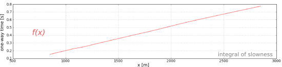
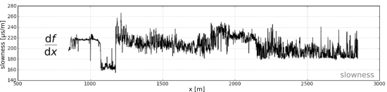
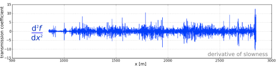
As far as I can tell, the well — despite usually being called "the Pechelbronn well" — was located at the site of a monument at the intersection of Route de Wœrth with Rue de Preuschdorf in Dieffenbach-lès-Wœrth, about 3 km west of Merkwiller-Pechelbronn. Henri Doll logged the well with Roger Jost and Charles Scheibli. Using rudimentary equipment, they logged about 145 m of the 488-metre hole, starting at 279 m MD, taking a reading every metre and plotting the log by hand. Yesterday I digitized this log; download it in LAS format here


Pechelbronn_thumbnail.png

The story of what the Schlumberger brothers and Henri Doll achieved is fascinating; I recommend reading Don Hill's brief history (2012) — it's free to read at Wiley. The period of invention that followed the Pechelbronn success was inspiring.

If you're looking at well logs today, take a second to thank Conrad, Maurice, and Henri for their remarkable idea.

PS If you're interested in petroleum history, the AOGHS page This Week is worth a look.


The French television programme Midi en France recorded this segment about the Pechelbronn field in 2014. The narration is in French, "The fields of maize gorge on sunshine, the pumps on petroleum...", but there are some nice pictures to look at.

References and bibliography

Clapp, Frederick G (1932). Oil and gas possibilities of France. AAPG Bulletin 16 (11), 1092–1143. Contains a good history of exploration and production from the Oligocene sands in Pechelbronn, up to about 1931 (the field produced up to 1970). AAPG Datapages.

Delacour, Jacques (2003). Une technique de prospection minière et pétrolière née en Pays d'Auge. SABIX 34, September 2003. Available online.

École des Mines page on Conrad Schlumberger at annales.org.

Hill, DG (2012). Appendix A: Historical Review (Milestone Developments in Petrophysics). In: Buryakovsky, L, Chilingar, GV, Rieke, HH, and Shin, S (2012). Petrophysics: Fundamentals of the Petrophysics of Oil and Gas Reservoirs, John Wiley & Sons, Inc., Hoboken, NJ, USA. doi: 10.1002/9781118472750.app1. A nice potted history of well logging, including important dates.

Musée Français du Pétrole website, http://www.musee-du-petrole.com/historique/

Pike, B and Duey, R (2002). Logging history rich with innovation. Hart's E&P Magazine. September 2002. Available online. Interesting article, but beware: there are one or two inaccuracies in this article, and I believe the image of the well log is incorrect.

Welly to the wescue

I apologize for the widiculous title.

Last week I described some headaches I was having with well data, and I introduced welly, an open source Python tool that we've built to help cure the migraine. The first versions of welly were built — along with the first versions of striplog — for the Nova Scotia Department of Energy, to help with their various data wrangling efforts.

Aside — all software projects funded by government should in principle be open source.

Today we're using welly to get data out of LAS files and into so-called feature vectors for a machine learning project we're doing for Canstrat (kudos to Canstrat for their support for open source software!). In our case, the features are wireline log measurements. The workflow looks something like this:

  1. Read LAS files into a welly 'project', which contains all the wells. This bit depends on lasio.
  2. Check what curves we have with the project table I showed you on Thursday.
  3. Check curve quality by passing a test suite to the project, and making a quality table (see below).
  4. Fix problems with curves with whatever tricks you like. I'm not sure how to automate this.
  5. Export as the X matrix, all ready for the machine learning task.

Let's look at these key steps as Python code.

1. Read LAS files

 
from welly import Project
p = Project.from_las('data/*.las')

2. Check what curves we have

Now we have a project full of wells and can easily make the table we saw last week. This time we'll use aliases to simplify things a bit — this trick allows us to refer to all GR curves as 'Gamma', so for a given well, welly will take the first curve it finds in the list of alternatives we give it. We'll also pass a list of the curves (called keys here) we are interested in:

The project table. The name of the curve selected for each alias is selected. The mean and units of each curve are shown as a quick QC. A couple of those RHOB curves definitely look dodgy, and they turned out to be DRHO correction curves.

The project table. The name of the curve selected for each alias is selected. The mean and units of each curve are shown as a quick QC. A couple of those RHOB curves definitely look dodgy, and they turned out to be DRHO correction curves.

3. Check curve quality

Now we have to define a suite of tests. Lists of test to run on each curve are held in a Python data structure called a dictionary. As well as tests for specific curves, there are two special test lists: Each and All, which are run on each curve encountered, and on all curves together, respectively. (The latter is required to, for example, compare the curves to each other to look for duplicates). The welly module quality contains some predefined tests, but you can also define your own test functions — these functions take a curve as input, and return either True (for a test pass) for False.

 
import welly.quality as qty
tests = {
    'All': [qty.no_similarities],
    'Each': [qty.no_monotonic],
    'Gamma': [
        qty.all_positive,
        qty.mean_between(10, 100),
    ],
    'Density': [qty.mean_between(1000,3000)],
    'Sonic': [qty.mean_between(180, 400)],
    }

html = p.curve_table_html(keys=keys, alias=alias, tests=tests)
HTML(html)
the green dot means that all tests passed for that curve. Orange means some tests failed. If all tests fail, the dot is red. The quality score shows a normalized score for all the tests on that well. In this case, RHOB and DT are failing the 'mean_b…

the green dot means that all tests passed for that curve. Orange means some tests failed. If all tests fail, the dot is red. The quality score shows a normalized score for all the tests on that well. In this case, RHOB and DT are failing the 'mean_between' test because they have Imperial units.

4. Fix problems

Now we can fix any problems. This part is not yet automated, so it's a fairly hands-on process. Here's a very high-level example of how I fix one issue, just as an example:

 
def fix_negs(c):
    c[c < 0] = np.nan
    return c

# Glossing over some details, we give a mnemonic, a test
# to apply, and the function to apply if the test fails.
fix_curve_if_bad('GAM', qty.all_positive, fix_negs)

What I like about this workflow is that the code itself is the documentation. Everything is fully reproducible: load the data, apply some tests, fix some problems, and export or process the data. There's no need for intermediate files called things like DT_MATT_EDIT or RHOB_DESPIKE_FINAL_DELETEME. The workflow is completely self-contained.

5. Export

The data can now be exported as a matrix, specifying a depth step that all data will be interpolated to:

 
X, _ = p.data_as_matrix(X_keys=keys, step=0.1, alias=alias)

That's it. We end up with a 2D array of log values that will go straight into, say, scikit-learn*. I've omitted here the process of loading the Canstrat data and exporting that, because it's a bit more involved. I will try to look at that part in a future post. For now, I hope this is useful to someone. If you'd like to collaborate on this project in the future — you know where to find us.

* For more on scikit-learn, don't miss Brendon Hall's tutorial in October's Leading Edge.


I'm happy to let you know that agilegeoscience.com and agilelibre.com are now served over HTTPS — so connections are private and secure by default. This is just a matter of principle for the Web, and we go to great pains to ensure our web apps modelr.io and pickthis.io are served over HTTPS. Find out more about SSL from DigiCert, the provider of Squarespace's (and Agile's) certs, which are implemented with the help of the non-profit Let's Encrypt, who we use and support with dollars.

Well data woes

I probably shouldn't be telling you this, but we've built a little tool for wrangling well data. I wanted to mention it, becase it's doing some really useful things for us — and maybe it can help you too. But I probably shouldn't because it's far from stable and we're messing with it every day.

But hey, what software doesn't have a few or several or loads of bugs?

Buggy data?

It's not just software that's buggy. Data is as buggy as heck, and subsurface data is, I assert, the buggiest data of all. Give units or datums or coordinate reference systems or filenames or standards or basically anything at all a chance to get corrupted in cryptic ways, and they take it. Twice if possible.

By way of example, we got a package of 10 wells recently. It came from a "data management" company. There are issues... Here are some of them:

  • All of the latitude and longitude data were in the wrong header fields. No coordinate reference system in sight anywhere. This is normal of course, and the only real side-effect is that YOU HAVE NO IDEA WHERE THE WELL IS.
  • Header chaos aside, the files were non-standard LAS sort-of-2.0 format, because tops had been added in their own little completely illegal section. But the LAS specification has a section for stuff like this (it's called OTHER in LAS 2.0).
  • Half the porosity curves had units of v/v, and half %. No big deal...
  • ...but a different half of the porosity curves were actually v/v. Nice.
  • One of the porosity curves couldn't make its mind up and changed scale halfway down. I am not making this up.
  • Several of the curves were repeated with other names, e.g. GR and GAM, DT and AC. Always good to have a spare, if only you knew if or how they were different. Our tool curvenam.es tries to help with this, but it's far from perfect.
  • One well's RHOB curve was actually the PEF curve. I can't even...

The remarkable thing is not really that I have this headache. It's that I expected it. But this time, I was out of paracetamol.

Cards on the table

Our tool welly, which I stress is very much still in development, tries to simplify the process of wrangling data like this. It has a project object for collecting a lot of wells into a single data structure, so we can get a nice overview of everything: 

Click to enlarge.

Our goal is to include these curves in the training data for a machine learning task to predict lithology from well logs. The trained model can make really good lithology predictions... if we start with non-terrible data. Next time I'll tell you more about how welly has been helping us get from this chaos to non-terrible data.

The calculus of geology

Calculus is the tool for studying things that change. Even so, in the midst of the dynamic and heterogeneous earth, calculus is an under-practised and, around the water-cooler at least, under-celebrated workhorse. Maybe that's because people don't realize it's all around us. Let's change that. 

Derivatives of duration

We can plot the time f(x) that passes as a seismic wave travels though space x. This function is known to many geophysicists as the time-to-depth function. It is key for converting borehole measurements, effectively recorded using a measuring tape, to seismic measurements, recorded using a stop watch.

Now let's take the derivative of f(x) with repsect to x. The result is the slowness function (the reciprocal of interval velocity):

The time duration that a seismic wave travels over a small interval (one metre). This function is an actual sonic well log. Differentiating once again yields this curious spiky function:

Geophysicists will spot that this resembles a reflection coefficient series, which governs seismic amplitudes. This is actually a transmission coefficient function, but that small detail is beside the point. In this example, the creating a synthetic seismogram mimics the calculus of geology. 

If you are familiar with the integrated trace attribute, you will recognize that it is an attempt to compute geology by integrating reflectivity spikes. The only issue in this case, and it is a major issue, is that the seismic trace is bandlimited. It does not contain all the information about the earth's slowness. So the earth's geology remains elusive and blurry.

The derivative of slowness yields the reflection boundaries, the integral of slowness yields their position. So in geophysics speak, I wonder, is forward modeling akin to differentiation, and inverse modeling akin to integration? I find it fascinating that these three functions have essentially the same density of information, yet they look increasingly complicated when we take derivatives. 

What other functions do you come across that might benefit from the calculus treatment?

The sonic log used in this example is from the O-32-B/11-E-64 well onshore Nova Scotia, which is publically available but not easily accessible online.

What is spectral gamma-ray?

The spectral gamma-ray log is a measure of the natural radiation in rocks. The amplitude of the signal from the gamma-ray tool, which is just a sensor with no active source, is proportional to the energy of the gamma-ray photons it encounters. Being able to differentiate between photons of different energies turns out to be very handy Compared to the ordinary gamma-ray log, which ignores the energies and only counts the photons, it's like seeing in colour instead of black and white.

Why do we care about gamma radiation?

First, what are gamma rays? Highly energetic photons: electromagnetic radiation with very short wavelengths. 

Being able to see different energies, or 'colours', means we can differentiate between the radioactive decay of different elements. Elements decay by radiating energy, and the 'colour' of that energy is characteristic of that element (actually, of each isotope). So, we can tell by looking at the energy of a photon if we are seeing a potassium atom (40K) or a uranium atom (238U) decay. These are very different isotopes, with very different habits. We can do geology!

In fact, all sorts of radioisotopes occur naturally in the earth. By far the most abundant are potassium 40K, thorium 232Th and uranium 238U. Of these, potassium is the most abundant in sedimentary rocks, but thorium and uranium are present in small quantities, and have particular sedimentological implications.

What exactly are we measuring?

Potassium 40K decays to argon about 10% of the time, with γ-emission at 1.46 MeV (the other 90% of the time it decays to calcium). However, all of the decay in the 232Th and 238U decay series occurs by α- and β-particle decay, which don't always result in photon emission. The tool in fact measures γ-radiation from the decay of thallium 208Tl in the 232Th series (right), and from bismuth 214Bi in the 238U series. The spectral gamma-ray tool must be calibrated to known samples to give concentrations of 232Th and 238U from its readings. Proper calibration is vital, and is temperature-sensitive (of note in Canada!).

The concentrations of the three elements are estimated from the spectral measure­ments. The concentration of potassium is usually measured in percent (%) or per mil (‰), or sometimes in kilograms per tonne, which is equivalent to per mil. The other two elements are measured in parts per million (ppm).

Here is the gamma-ray spectrum from a single sample from 509 m below the sea-floor at ODP Site 1201. The final spectrum (heavy black line) is shown after removing the background spectrum (gray region) and applying a three-point mean boxcar filter. The thin black line shows the raw spectrum. Vertical lines mark the interval boundaries defined by Peter Blum (an ODP scientist at Texas A&M). Prominent energy peaks relating to certain elements are identified at the top of the figure. The inset shows the spectrum for energies >1500 keV at an expanded scale. 

We wouldn't normally look at these spectra. Instead, the tool provides logs for K, Th, and U. Next time, I'll look at the logs.

Spectrum illustration by Wikipedia user Inductiveload, licensed GFDL; decay chain by Wikipedia user BatesIsBack, licensed CC-BY-SA.

Rocks, pores and fluids

At an SEG seismic rock physics conference in China several years ago, I clearly remember a catch phrase used by one of the presenters, "It's all about rocks, pores, and fluids." He used it several times throughout his talk as an invocation for geophysicists to translate their seismic measurements of the earth into terms that are more appealing to others. Nobody cares about the VP/VS ratio in a reservoir. Even though I found the repetition slightly off-putting, he succeeded—the phrase stuck. It's all about rock, pores, and fluids.

Fast forward to the SEG IQ Earth Forum a few months ago. The message reared its head again, but in a different form. After dinner one evening, I was speaking with Ran Bachrach about advances in seismic rock physics technology: the glamour and the promise of the state-of-the-art. It was a topic right up his alley, but suprisingly, he seemed ambivalent and under-enthused. Which was unusual for him. "More often than not," he said, "we can get all the information we need from the triple combo." 

What is the triple combo? 

I felt embarrased that I had never heard of the term. Like I had been missing something this whole time. The triple combo is the standard set of measurements used in formation evaluation and wireline logging: gamma-ray, porosity, and resistivity. Simply put, the triple combo tells us about rocks, pores, and fluids. 

I find it curious that the very things we are interested in are impossible to measure directly. For example:

  • A gamma-ray log measures naturally occuring radioactive minerals. We use this to make inferences about lithology.
  • A neutron log measures Compton scattering in proportion to the number of hydrogen atoms. This is a proxy for pores.
  • A resistivity log measures the conductivity of electrical current. We use this to tell us about fluid type and saturation.

Subsurface geotechnology isn't only about recording the earth's constituents in isolation. Some measurements, the sonic log for instance, are useful because of the fact that they are an aggregate of all three.

The well log is a section of the Thebaud_E-74 well available from the offshore Nova Scotia Play Fairway Analysis.

Cope don't fix

Some things genuinely are broken. International financial practices. Intellectual property law. Most well tie software. 

But some things are the way they are because that's how people like them. People don't like sharing files, so they stash their own. Result: shared-drive cancer — no, it's not just your shared drive that looks that way. The internet is similarly wild, chaotic, and wonderful — but no-one uses Yahoo! Directory to find stuff. When chaos is inevitable, the only way to cope is fast, effective search

So how shall we deal with the chaos of well log names? There are tens of thousands — someone at Schlumberger told me last week that they alone have over 50,000 curve and tool names. But these names weren't dreamt up to confound the geologist and petrophysicist — they reflect decades of tool development and innovation. There is meaning in the morasse.

Standards are doomed

Twelve years ago POSC had a go at organizing everything. I don't know for sure what became of the effort, but I think it died. Most attempts at standardization are doomed. Standards are awash with compromise, so they aren't perfect for anything. And they can't keep up with changes in technology, because they take years to change. Doomed.

Instead of trying to fix the chaos, cope with it.

A search tool for log names

We need a search tool for log names. Here are some features it should have:

  • It should be free, easy to use, and fast
  • It should contain every log and every tool from every formation evaluation company
  • It should provide human- and machine-readable output to make it more versatile
  • You should get a result for every search, never drawing a blank
  • Results should include lots of information about the curve or tool, and links to more details
  • Users should be able to flag or even fix problems, errors, and missing entries in the database

To my knowledge, there are only two tools a little like this: Schlumberger's Curve Mnemonic Dictionary, and the SPWLA's Mnemonics Data Search. Schlumberger's widget only includes their tools, naturally. The SPWLA database does at least include curves from Baker Hughes and Halliburton, but it's at least 10 years out of date. Both fail if the search term is not found. And they don't provide machine-readable output, only HTML tables, so it's difficult to build a service on them.

Introducing fuzzyLAS

We don't know how to solve this problem, but we're making a start. We have compiled a database containing 31,000 curve names, and a simple interface and web API for fuzzily searching it. Our tool is called fuzzyLAS. If you'd like to try it out, please get in touch. We'd especially like to hear from you if you often struggle with rogue curve mnemonics. Help us build something useful for our community.

The digital well scorecard

In my last post, I ranted about the soup of acronyms that refer to well log curves; a too-frequent book-keeping debacle. This pain, along with others before it, has motivated me to design a solution. At this point all I have is this sketch, a wireframe of should-be software that allows you visualize every bit of borehole data you can think of:

The goal is, show me where the data is in the domain of the wellbore. I don't want to see the data explicitly (yet), just its whereabouts in relation to all other data. Data from many disaggregated files, reports, and so on. It is part inventory, part book-keeping, part content management system. Clear the fog before the real work can begin. Because not even experienced folks can see clearly in a fog.

The scorecard doesn't yield a number or a grade point like a multiple choice test. Instead, you build up a quantitative display of your data extents. With the example shown above, I don't even have to look at the well log to tell you that you are in for a challenging well tie, with the absence of sonic measurements in the top half of the well. 

The people that I showed this to immediately undestood what was being expressed. They got it right away, so that bodes well for my preliminary sketch. Can you imagine using a tool like this, and if so, what features would you need? 

Swimming in acronym soup

In a few rare instances, an abbreviation can become so well-known that it is adopted into everyday language; more familar than the words it used to stand for. It's embarrasing, but I needed to actually look up LASER, and you might feel the same way with SONAR. These acronyms are the exception. Most are obscure barriers to entry in technical conversations. They can be constructs for wielding authority and exclusivity. Welcome to the club, if you know the password.

No domain of subsurface technology is riddled with more acronyms than well log analysis and formation evaluation. This is a big part of — perhaps too much of a part of — why petrophysics is hard. Last week, I came across a well. It has an extended suite of logs, and I wanted make a synthetic. Have a glance at the image and see which curve names you recognize (the size represents the frequency the names are encountered across many files of the same well).

I felt like I was being spoken to by some earlier deliquent: I got yer well logs right here buddy. Have fun sorting this mess out.

The log ASCII standard (*.LAS file) file format goes a long way to exposing descriptive information in the header. But this information is often incomplete, missing, and says nothing about the quality or completeness of the data. I had to scan 5 files to compile this soup. A micro-travesty and a failure, in my opinion. How does one turn this into meaningful information for geoscience?

Whose job is it to sort this out? The service company that collected the data? The operator that paid for it? A third party down the road?

What I need is not only an acronym look-up table, but also a data range tool to show me what I've got in the file (or files), and at which locations and depths I've got it. A database to give me more information about these acronyms would be nice too, and a feature that allows me to compare multiple files, wells, and directories at once. It would be like a life preserver. Maybe we should build it.

I made the word cloud by pasting text into wordle.net. I extracted the text from the data files using the wonderful LASReader written by Warren Weckesser. Yay, open source!

Bring it into time

A student competing in the AAPG's Imperial Barrel Award recently asked me how to take seismic data, and “bring it into depth”. How I read this was, “how do I take something that is outside my comfort zone, and make it fit with what is familiar?” Geologists fear the time domain. Geology is in depth, logs are in depth, drill pipe is in depth. Heck, even X and Y are in depth. Seismic data relates to none of those things; useless right? 

It is excusable for the under-initiated, but this concept of “bringing [time domain data] into depth” is an informal fallacy. Experienced geophysicists understand this because depth conversion, in all of its forms and derivatives, is a process that introduces a number of known unknowns. It is easier for others to be dismissive, or ignore these nuances. So early-onset discomfort with the travel-time domain ensues. It is easier to stick to a domain that doesn’t cause such mental backflips; a kind of temporal spatial comfort zone. 

Linear in time

However, the unconverted should find comfort in one property where the time domain is advantageous; it is linear. In contrast, many drillers and wireline engineers are quick to point that measured depth is not nessecarily linear. Perhaps time is an even more robust, more linear domain of measurement (if there is such a concept). And, as a convenient result, a world of possibilities emerge out of time-linearity: time-series analysis, digital signal processing, and computational mathematics. Repeatable and mechanical operations on data.

Boot camp in time

The depth domain isn’t exactly omnipotent. A colleague, who started her career as a wireline-engineer at Schlumberger, explained to me that her new-graduate training involved painfully long recitations and lecturing on the intricacies of depth. What is measured depth? What is true vertical depth? What is drill-pipe stretch? What is wireline stretch? And so on. Absolute depth is important, but even with seemingly rigid sections of solid steel drill pipe, it is still elusive. And if any measurement requires a correction, that measurement has error. So even working in the depth domain data has its peculiarities.

Few of us ever get the privilege of such rigorous training in the spread of depth measurements. Sitting on the back of the rhetorical wireline truck, watching the coax-cable unpeel into the wellhead. Few of us have lifted a 300 pound logging tool, to feel the force that it would impart on kilometres of cable. We are the recipients of measurements. Either it is a text file, or an image. It is what it is, and who are we to change it? What would an equvialent boot camp for travel-time look like? Is there one?

In the filtered earth, even the depth domain is plastic. Travel-time is the only absolute.