x lines of Python: AVO plot

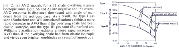
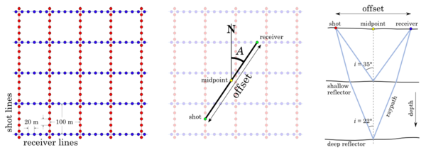
Amplitude vs offset (or, more properly, angle) analysis is a core component of quantitative interpretation. The AVO method is based on the fact that the reflectivity of a geological interface does not depend only on the acoustic rock properties (velocity and density) on both sides of the interface, but also on the angle of the incident ray. Happily, this angular reflectivity encodes elastic rock property information. Long story short: AVO is awesome.

As you may know, I'm a big fan of forward modeling — predicting the seismic response of an earth model. So let's model the response the interface between a very simple model of only two rock layers. And we'll do it in only a few lines of Python. The workflow is straightforward:

1. Define the properties of a model shale; this will be the upper layer.
2. Define a model sandstone with brine in its pores; this will be the lower layer.
3. Define a gas-saturated sand for comparison with the wet sand. 
4. Define a range of angles to calculate the response at.
5. Calculate the brine sand's response at the interface, given the rock properties and the angle range.
6. For comparison, calculate the gas sand's response with the same parameters.
7. Plot the brine case.
8. Plot the gas case.
9. Add a legend to the plot.

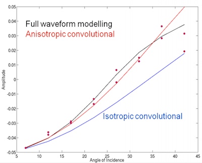
That's it — nine lines! Here's the result:

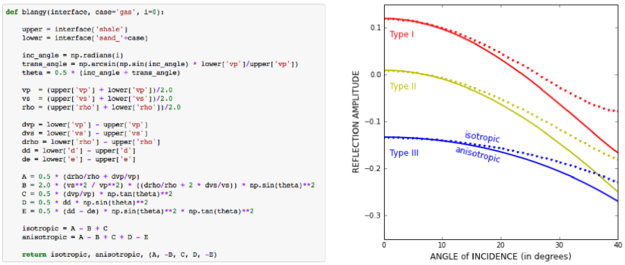
Once we have rock properties, the key bit is in the middle:

    θ = range(0, 31)
    shuey = bruges.reflection.shuey2(vp0, vs0, ρ0, vp1, vs1, ρ1, θ)

shuey2 is one of the many functions in bruges — here it provides the two-term Shuey approximation, but it contains lots of other useful equations. Virtually everything else in our AVO plotting routine is just accounting and plotting.

---

As in all these posts, you can follow along with the code in the Jupyter Notebook. You can view this on GitHub, or run it yourself in the increasingly flaky MyBinder (which is down at the time of writing... I'm working on an alternative).

What would you like to see in x lines of Python? Requests welcome!

What is AVO-friendly processing?

It's the Geophysics Hackathon next month! Come down to Propeller in New Orleans on 17 and 18 October, and we'll feed you and give you space to build something cool. You might even win a prize. Sign up — it's free!

Thank you to the sponsors, OpenGeoSolutions and Palladium Consulting — both fantastic outfits. Hire them.

AVO-friendly processing gets called various things: true amplitude, amplitude-friendly, and controlled amplitude, controlled phase (or just 'CACP'). And, if you've been involved in any processing jobs you'll notice these phrases get thrown around a lot. But seismic geophysics has a dirty little secret... we don't know exactly what it is. Or, at least, we can't agree on it.

A LinkedIn discussion in the Seismic Data Processing group earlier this month prompted this post:

I can't compile a list of exactly which processes will harm your AVO analysis (can anyone? Has anyone??), but I think I can start a list of things that you need to approach with caution and skepticism:

• Anything that is not surface consistent. What does that mean? According to Oliver Kuhn (now at Quantec in Toronto):

Surface consistent: a shot-related [process] affects all traces within a shot gather in the same way, independent of their receiver positions, and, a receiver-related [process] affects all traces within a receiver gather in the same way, independent of their shot positions.

• Anything with a window — spatial or temporal. If you must use windows, make them larger or longer than your areas and zones of interest. In this way, relative effects should be preserved.
• Anything that puts the flattening of gathers before the accuracy of the data (<cough> trim statics). Some flat gathers don't look flat. (The thumbnail image for this post is from Duncan Emsley's essay in 52 Things.)
• Anything that is a sort of last resort, post hoc attempt to improve the data — what we might call 'cosmetic' treatments. Things like wavelet stretch correction and spectral shaping are good for structural interpreters, but not for seismic analysts. At the very least, get volumes without them, and convince yourself they did no harm.
• Anything of which people say, "This should be fine!" but offer no evidence.

Back to my fourth point there... spectral shaping and wavelet stretch correction (e.g. this patented technique I was introduced to at ConocoPhillips) have been the subject of quite a bit of discussion, in my experience. I don't know why; both are fairly easy to model, on the face of it. The problem is that we start to get into the sticky question of what wavelets 'see' and what's a wavelet anyway, and hang on a minute why does seismic reflection even work? Personally, I'm skeptical, especially as we get more used to, and better at, looking at spectral decompositions of stacked and pre-stack data.

Divergent paths

I have seen people use seismic data with very different processing paths for structural interpretation and for AVO analysis. This can happen on long-term projects, where the structural framework depends on an old post-stack migration that was later reprocessed for AVO friendliness. This is a bad idea — you won't be able to put the quantitative results into the structural framework without introducing substantial error.

What we need is a clinical trial of processing algorithms, in which they are tested against a known model like Marmousi, and their effect on attributes is documented. If such studies exist, I'd love to hear about them. Come to think of it, this would make a good topic for a hackathon some day... Maybe Dallas 2016?

The Blangy equation

After reading Chris Liner's recent writings on attenuation and negative Q — both in The Leading Edge and on his blog — I've been reading up a bit on anisotropy. The idea was to stumble a little closer to writing the long-awaited Q is for Q post in our A to Z series. As usual, I got distracted...

In his 1994 paper AVO in tranversely isotropic media—An overview, Blangy (now the chief geophysicist at Hess) answered a simple question: How does anisotropy affect AVO? Stigler's law notwithstanding, I'm calling his solution the Blangy equation. The answer turns out to be: quite a bit, especially if impedance contrasts are low. In particular, Thomsen's parameter δ affects the AVO response at all offsets (except zero of course), while ε is relatively negligible up to about 30°.

The key figure is Figure 2. Part (a) shows isotropic vs anisotropic Type I, Type II, and Type III responses:

Unpeeling the equation

Converting the published equation to Python was straightforward (well, once Evan pointed out a typo — yay editors!). Here's a snippet, with the output (here's all of it):

For the plot below, I computed the terms of the equation separately for the Type II case. This way we can see the relative contributions of the terms. Note that the 3-term solution is equivalent to the Aki–Richards equation.

Interestingly, the 5-term result is almost the same as the 2-term approximation.

Reproducible results

One of the other nice features of this paper — and the thing that makes it reproducible — is the unambiguous display of the data used in the models. Often, this sort of thing is buried in the text, or not available at all. A table makes it clear:

Last thought: is it just me, or is it mind-blowing that this paper is now over 20 years old?

Reference

Blangy, JP (1994). AVO in tranversely isotropic media—An overview. Geophysics 59 (5), 775–781.

Don't miss the IPython Notebook that goes with this post.

O is for Offset

Offset is one of those jargon words that geophysicists kick around without a second thought, but which might bewilder more geological interpreters. Like most jargon words, offset can mean a couple of different things: 

• Offset distance, which is usually what is meant by simply 'offset'.
• Offset angle, which is often what we really care about.
• We are not talking about offset wells, or fault offset.

What is offset?

Sherriff's Encyclopedic Dictionary is characteristically terse:

Offset: The distance from the source point to a geophone or to the center of a geophone group.

The concept of offset only really makes sense in the pre-stack world — to field data and gathers. The traces in stacked data (everyday seismic volumes) combine data from many offsets. So let's look at the geometry of seismic acquisition. A map shows the layout of shots (red) and receivers (blue). We can define offset and azimuth A at the midpoint of every shot–receiver pair, on a map (centre) and in section (right):

Offset distance applies to traces. The offset distance is the straight-line distance from the vibrator, shot-hole or air-gun (or any other source) to the particular receiver that recorded the trace in question. If we know the geometry of the acquisition, and the size of the recording patch or length of the streamers, then we can calculate offset distance exactly. 

Offset angle applies to specific samples on a trace. The offset angle is the incident angle of the reflected ray that that a given sample represents. Samples at the top of a trace have larger offset angles than those at the bottom, even though they have the same offset distance. To compute these angles, we need to know the vertical distances, and this requires knowledge of the velocity field, which is mostly unknown. So offset angle is not objective, but a partly interpreted quantity.

Why do we care?

Acquiring longer offsets can help undershoot gaps in a survey, or image beneath salt canopies and other recumbent features. Longer offsets also helps with velocity estimation, because we see more moveout.

Looking at how the amplitude of a reflection changes with offset is the basis of AVO analysis. AVO analysis, in turn, is the basis of many fluid and lithology prediction techniques.

Offset is one of the five canonical dimensions of pre-stack seismic data, along with inline, crossline, azimuth, and frequency. As such, it is a key part of the search for sparsity in the 5D interpolation method perfected by Daniel Trad at CGGVeritas. 

Recently, geophysicists have become interested not just in the angle of a reflection, but in the orientation of a reflection too. This is because, in some geological circumstances, the amplitude of a reflection depends on the orientation with respect to the compass, as well as the incidence angle. For example, looking at data in both of these dimensions can help us understand the earth's stress field.

Offset is the characteristic attribute of pre-stack seismic data. Seismic data would be nothing without it.

Ten ways to spot pseudogeophysics

Geophysicists often try to predict rock properties using seismic attributes — an inverse problem. It is difficult and can be complicated. It can seem like black magic, or at least a black box. They can pull the wool over their own eyes in the process, so don’t be surprised if it seems like they are trying to pull the wool over yours. Instead, ask a lot of questions.

Questions to ask

1. What is the reliability of the logs that are inputs to the prediction? Ask about hole quality and log editing.
2. What about the the seismic data? Ask about signal:noise, multiples, bandwidth, resolution limits, polarity, maximum offset angle (for AVO studies), and processing flow (e.g. Emsley, 2012).
3. What is the quality of the well ties? Is the correlation good enough for the proposed application?
4. Is there any physical reason why the seismic attribute should predict the proposed rock property? Was this explained to you? Were you convinced?
5. Is the proposed attribute redundant (sensu Barnes, 2007)? Does it really give better results than a less sexy approach? I’ve seen 5-minute trace integration outperform month-long AVO inversions (Hall et al. 2006).
6. What are the caveats and uncertainties in the analysis? Is there a quantitative, preferably Bayesian, treatment of the reliability of the predictions being made? Ask about the probability of a prediction being wrong.
7. Is there a convincing relationship between the rock property (shear impedance, say) and some geologically interesting characteristic that you actually make decisions with, e.g. frackability.
8. Is there a convincing relationship between the rock property and the seismic attribute at the wells? In other words, does the attribute actually correlate with the property where we have data?
9. What does the low-frequency model look like? How was it made? Its maximum frequency should be about the same as the seismic data's minimum, no more.
10. Does the geophysicist compute errors from the training error or the validation error? Training errors are not helpful because they beg the question by comparing the input training data to the result you get when you use those very data in the model. Funnily enough, most geophysicists like to show the training error (right), but if the model is over-fit then of course it will predict very nicely at the well! But it's the reliability away from the wells we are interested in, so we should examine the error we get when we pretend the well isn't there. I prefer this to witholding 'blind' wells from the modeling — you should use all the data. 

Lastly, it might seem harsh but we could also ask if the geophysicist has a direct financial interest in convincing you that their attribute is sound, as well as the normal direct professional interest. It’s not a problem if they do, but be on your guard — people who are selling things are especially prone to bias. It's unavoidable.

What do you think? Are you bamboozled by the way geophysicists describe their predictions?

References
Barnes, A (2007). Redundant and useless seismic attributes. Geophysics 72 (3), p P33–P38. DOI: 10.1190/1.2370420.
Emsley, D. Know your processing flow. In: Hall & Bianco, eds, 52 Things You Should Know About Geophysics. Agile Libre, 2012. 
Hall, M, B Roy, and P Anno (2006). Assessing the success of pre-stack inversion in a heavy oil reservoir: Lower Cretaceous McMurray Formation at Surmont. Canadian Society of Exploration Geophysicists National Convention, Calgary, Canada, May 2006. 

The image of the training error plot — showing predicted logs in red against input logs — is from Hampson–Russell's excellent EMERGE software. I'm claiming the use of the copyrighted image is fair use.  

Resolution, anisotropy, and brains

Day 1 of the SEG Annual Meeting continued with the start of the regular program — 96 talks and 71 posters, not to mention the 323 booths on the exhibition floor. Instead of deciding where to start, I wandered around the bookstore and bought Don Herron's nice-looking new book, First Steps in Seismic Interpretation, which we will review some time soon.

Here are my highlights from the rest of the day.

Chuck Ursenbach, Arcis

Calgary is the home of seismic geophysics. There's a deep tradition of signal processing, and getting the basics right. Sometimes there's snake oil too, but mostly it's good, honest science. And mathematics. So when Jim Gaiser suggested last year at SEG that PS data might offer as good resolution as SS or PP — as good, and possibly better — you know someone in Calgary will jump on it with MATLAB. Ursenbach, Cary, and Perz [PDF] did some jumping, and conclude: PP-to-PS mapping can indeed increase bandwidth, but the resolution is unchanged, because the wavelength is unchanged — 'conservation of resolution', as Ursenbach put it. Resolution isn't everything. 

Gabriel Chao, Total E&P

Chao showed a real-world case study starting with a PreSTM gather with a decent Class 2p AVO anomaly at the top of the reservoir interval (TTI Kirchhoff with 450–4350 m offset). There was residual NMO in the gather, as Leon Thomsen himself later forced Chao to admit, but there did seem to be a phase reversal at about 25°. The authors compared the gather with three synthetics: isotropic convolutional, anisotropic convolutional, and full waveform. The isotropic model was fair, but the phase reversal was out at 33°. The anisotropic convolutional model matched well right up to about 42°, beyond which only the full waveform model was close (right). Anisotropy made a similar difference to wavelet extraction, especially beyond about 25°.

Canada prevails

With no hockey to divert them, Canadians are focusing on geophysical contests this year. With the Canadian champions Keneth Silva and Abdolnaser Yousetz Zadeh denied the chance to go for the world title by circumstances beyond their control, Canada fielded a scratch team of Adrian Smith (U of C) and Darragh O'Connor (Dalhousie). So much depth is there in the boreal Americas that the pair stormed home with the trophy, the cash, and the glory.

The Challenge Bowl event was a delight — live music, semi-raucous cheering, and who can resist MC Peter Duncan's cheesy jests? If you weren't there, promise yourself you'll go next year. 

The image from Chao is copyright of SEG, from the 2012 Annual Meeting proceedings, and used here in accordance with their permissions guidelines. The image of Herron's book is also copyright of SEG; its use here is proposed to be fair use.

Quantifying the earth

I am in Avon, Colorado, this week attending the SEG IQ Earth Forum. IQ (integrative and quantitative) Earth is a new SEG committee formed in reponse to a $1M monetary donation by Statoil to build a publicly available, industrial strength dataset for the petroleum community. In addition to hosting a standard conference format of podiums and Q and A's, the SEG is using the forum to ask delegates for opinions on how to run the committee. There are 12 people in attendance from consulting & software firms, 11 from service companies, 13 who work for operators, and 7 from SEG and academia. There's lively discussionafter each presentation, which has twice been cut short by adherence to the all important 2 hour lunch break. That's a shame. I wish the energy was left to linger. Here is a recap of the talks that have stood out for me so far:

Yesterday, Peter Wang from WesternGeco presented 3 mini-talks in 20 minutes showcasing novel treatments of uncertainty. In the first talk he did a stochastic map migration of 500 equally probable anisotropic velocity models that translated a fault plane within a 800 foot lateral uncertainty corridor. The result was even more startling on structure maps. Picking a single horizon or fault is wrong, and he showed by how much. Secondly, he showed a stocastic inversion using core, logs and seismic. He again showed the results of hundreds of non-unique but equally probable inversion realizations, each exactly fit the well logs. His point: one solution isn't enough. Only when we compute the range of possible answers can we quantify risk and capture our unknowns. Third, he showed an example from a North American resource shale, a setting where seismic methods are routinely under-utilized, and ironically, a setting where 70% of the production comes from less than 30% of the completed intervals. The geomechanical facies classification showed compelling frac barriers and non reservoir classes, coupled to an all-important error cube, showing the probability of each classification, the confidence of the method.

Ron Masters, from a software company called Headwave, presented a pre-recorded video demonstration of his software in action. Applause goes to him for a pseudo-interactive presentation. He used horizons as a boundary for scuplting away peripheral data for 3D AVO visualizations. He demostrated the technique of rotating a color wheel in the intercept-gradient domain, such that any and all linear combinations of AVO parameters can be mapped to a particular hue. No more need for hard polygons. Instead, with gradational crossplot color classes, the AVO signal doesn't get suddenly clipped out, unless there is a real change in fluid and lithology effects. Exposing AVO gathers in this interactive environment guards against imposing false distinctions that aren’t really there. 

The session today consisted of five talks from WesternGeco / Schlumberger, a powerhouse of technology who stepped up to show their heft. Their full occupancy of the podium today, gives a new meaning to the rhyming quip; all-day Schlumberger. Despite having the bias of an internal company conference, it was still very entertaining, and informative. 

Andy Hawthorn showed how seismic images can be re-migrated around the borehole (almost) in real time by taking velocity measurements while drilling. The new measurements help drillers adjust trajectories and mud weights entering hazardous high pressure which has remarkable safety and cost benefits. He showed a case where a fault was repositioned by 1000 vertical feet; huge implications for wellbore stability, placing casing shoes, and other such mechanical considerations. His premise is that the only problem worth our attention is the following: it is expensive to drill and produce wells. Science should not be done for the sake of it; but to build usable models for drillers. 

In a characteristically enthusiastic talk, Ran Bachrach showed how he incorporated a compacting shale anisotropic rock physics model with borehole temperature and porosity measurements to expedite empirical hypothesis testing of imaging conditions. His talk, like many before him throughout the Forum, touched on the notion of generating many solutions, as fast as possible. Asking questions of the data, and being able to iterate. 

At the end of the first day, Peter Wang stepped boldy back to the to the microphone while others has started packing their bags, getting ready to leave the room. He commented that what an "integrated and quantitative" earth model desperately needs are financial models and simulations. They are what drive this industry; making money. As scientists and technologists we must work harder to demonstrate the cost savings and value of these techniques. We aren't getting the word out fast enough, and we aren't as relevant as we could be. It's time to make the economic case clear.

Your child is dense for her age

Alan Cohen, veteran geophysicist and Chief Scientist at RSI, secured the role of provacateur by posting this question on the rock physics group on LinkedIn. He has shown that the simplest concepts are worthy of debate.

From a group of 1973 members, 44 comments ensued over the 23 days since he posted it. This has got to be a record for this community (trust me I've checked). It turns out the community is polarized, and heated emotions surround the topic. The responses that emerged are a fascinating narrative of niche and tacit assumptions seldomly articulated.

Any two will do

Why are two dimensions used, instead of one, three, four, or more? Well for one, it is hard to look at scatter plots in 3D. More fundamentally, a key learning from the wave equation and continuum mechanics is that, given any two elastic properties, any other two can be computed. In other words, for any seismically elastic material, there are two degrees of freedom. Two parameters to describe it.

• P- and S-wave velocities
• P-impedance and S-impedance
• Acoustic and elastic impedance
• R₀ and G, the normal-incidence reflectivity and the AVO gradient
• Lamé's parameters, λ and μ 

Each pair has its time and place, and as far as I can tell there are reasons that you might want to re-parameterize like this:

1. one set of parameters contains discriminating evidence, not visible in other sets;
2. one set of parameters is a more intuitive or more physical description of the rock—it is easier to understand;
3. measurement errors and uncertainties can be elucidated better for one of the choices. 

Something missing from this thread, though, is the utility of empirical templates to makes sense of the data, whichever domain is adopted.

Measurements with a backdrop

In child development, body mass index (BMI) is plotted versus age to characterize a child's physical properties using the backdrop of an empirically derived template sampled from a large population. It is not so interesting to say, "13 year old Miranda has a BMI of 27", it is much more telling to learn that Miranda is above the 95th percentile for her age. But BMI, which is defined as weight divided by height squared, in not particularity intuitive. If kids were rocks, we'd submerge them Archimedes style into a bathtub, measure their volume, and determine their density. That would be the ultimate description. "Whoa, your child is dense for her age!" 

We do the same things with rocks. We algebraically manipulate measured variables in various ways to show trends, correlations, or clustering. So this notion of a template is very important, albeit local in scope. Just as a BMI template for Icelandic children might not be relevant for the pygmies in Paupa New Guinea, rock physics templates are seldom transferrable outside their respective geographic regions. 

For reference see the rock physics cheatsheet.

AVO* is free!

The two-bit experiment is over! We tried charging $2 for one of our apps, AVO*, as a sort of techno-socio-geological experiment, and the results are in: our apps want to be free. Here are our download figures, as of this morning: 

You also need to know when these apps came out. I threw some of the key statistics into SubSurfWiki and here's how they stack up when you account for how long they've been available:

It is clear that AVO* has performed quite poorly compared to its peers! The retention rate (installs/downloads) is 100% — the price tag buys you loyalty and even a higher perceived value perhaps? But the hit in adoption is too much to take. 

There are other factors: quality, relevance, usefulness, ease-of-use. It's hard to be objective, but I think AVO* is our highest quality app. It certainly has the most functionality, hence this experiment. It is rather niche: many geological interpreters may have no use for it. But it is certainly no more niche than Elastic*, and has about four times the functionality. On the downside, it needs an internet connection for most of its juicy bits.

In all, I think that we might have expected 200 installs for the app by now, from about 400–500 downloads. I conclude that charging $2 has slowed down its adoption by a factor of ten, and hereby declare it free for everyone. It deserves to be free! If you were one of the awesome early adopters that paid a toonie for it, I have only this to say to you: we love you.

So, if you have an Android device, scan the code or otherwise hurry to the Android Market!

What is AVO?

I used to be a geologist (but I'm OK now). When I first met seismic data, I took the reflections and geometries quite literally. The reflections come from geology, so it seems reasonable to interpret them as geology. But the reflections are waves, and waves are slippery things: they have to travel through kilometres of imperfectly known geology; they can interfere and diffract; they emanate spherically from the source and get much weaker quickly. This section from the Rockall Basin in the east Atlantic shows this attenuation nicely, as well as spectacular echo reflections from the ocean floor called multiples:

Data from the Virtual Seismic Atlas, contributed by the British Geological Survey.

Impedance is the product of density and velocity. Despite the complexity of seismic reflections, all is not lost. Even geologists interpreting seismic know that the strength of seismic reflections can have real, quantitative, geological meaning. For example, amplitude is related to changes in acoustic impedance Z, which is equal to the product of bulk density ρ and P-wave velocity V, itself related to lithology, fluid, and porosity.

Flawed cartoon of a marine seismic survey. OU, CC-BY-SA-NC.

But when the amplitude versus offset (AVO) behaviour of seismic reflections gets mentioned, most non-geophysicists switch off. If that's your reaction too, don't be put off by the jargon, it's really not that complicated.

The idea that we collect data from different angles is not complicated or scary. Remember the classic cartoon of a seismic survey (right). It's clear that some of the ray paths bounce off the geological strata at relatively small incidence angles, closer to straight down-and-up. Others, arriving at receivers further away from the source, have greater angles of incidence. The distance between the source and an individual receiver is called offset, and is deducible from the seismic field data because the exact location of the source and receivers is always known.

The basic physics behind AVO analysis is that the strength of a reflection does not only depend on the acoustic impedance—it also depends on the angle of incidence. Only when this angle is 0 (a vertical, or zero-offset, ray) does the simple relationship above hold.

Total internal reflection underwater. Source: Mbz1 via Wikimedia Commons.Though it may be unintuitive at first, angle-dependent reflectivity is an idea we all know well. Imagine an ordinary glass window: you can see through it perfectly well when you look straight through it, but when you move to a wide angle it suddenly becomes very reflective (at the so-called critical angle). The interface between water and air is similarly reflective at wide angles, as in this underwater view.

Karl Bernhard Zoeppritz (German, 1881–1908) was the first seismologist to describe the relationship between reflectivity and angle of incidence. In this context, describe means write down the equations for. Not two or three equations, lots of equations.

The Zoeppritz equations are very good model for how seismic waves propagate in the earth. There are some unnatural assumptions about isotropy, total isolation of the interface, and other things, but they work well in many real situations. The problem is that the equations are unwieldy, especially if you are starting from seismic data and trying to extract rock properties—trying to solve the so-called inverse problem. Since we want to be able to do useful things quickly, and since seismic data are inherently approximate anyway, several geophysicists have devised much friendlier models of reflectivity with offset.

I'll take a look at these more friendly models next time, because I want to tell a bit about how we've implemented them in our soon-to-be-released mobile app, AVO*. No equations, I promise! Well, one or two...