A (useless) map of geo-mathematics

Most scientific problems involve at least a bit of maths, even if it’s just adding things up or finding averages.

But some problems require quite a bit of maths, like solving an equation, or throwing vectors around, or even a Fourier transform or two. A lot of people switch off at this point.

Yet other problems require a lot of maths. Maybe we need a finite difference model, a volume integral, or a deep neural network. Most of us back away from the problem at this point and look for a collaborator with a lot of equations on their whiteboard.

But it’s pretty hard to find new collaborators right now. And what if you run into these problems a lot? Maybe you need to be the one with the equationy whiteboard!

What then? Where do you start? We need a map!

A roadmap for learning…

…is what I set out to draw. I failed. Possibly there exists a map, with START HERE in one corner and a whiteboard full of equations in the other. But I doubt it.

I ended up drawing this:

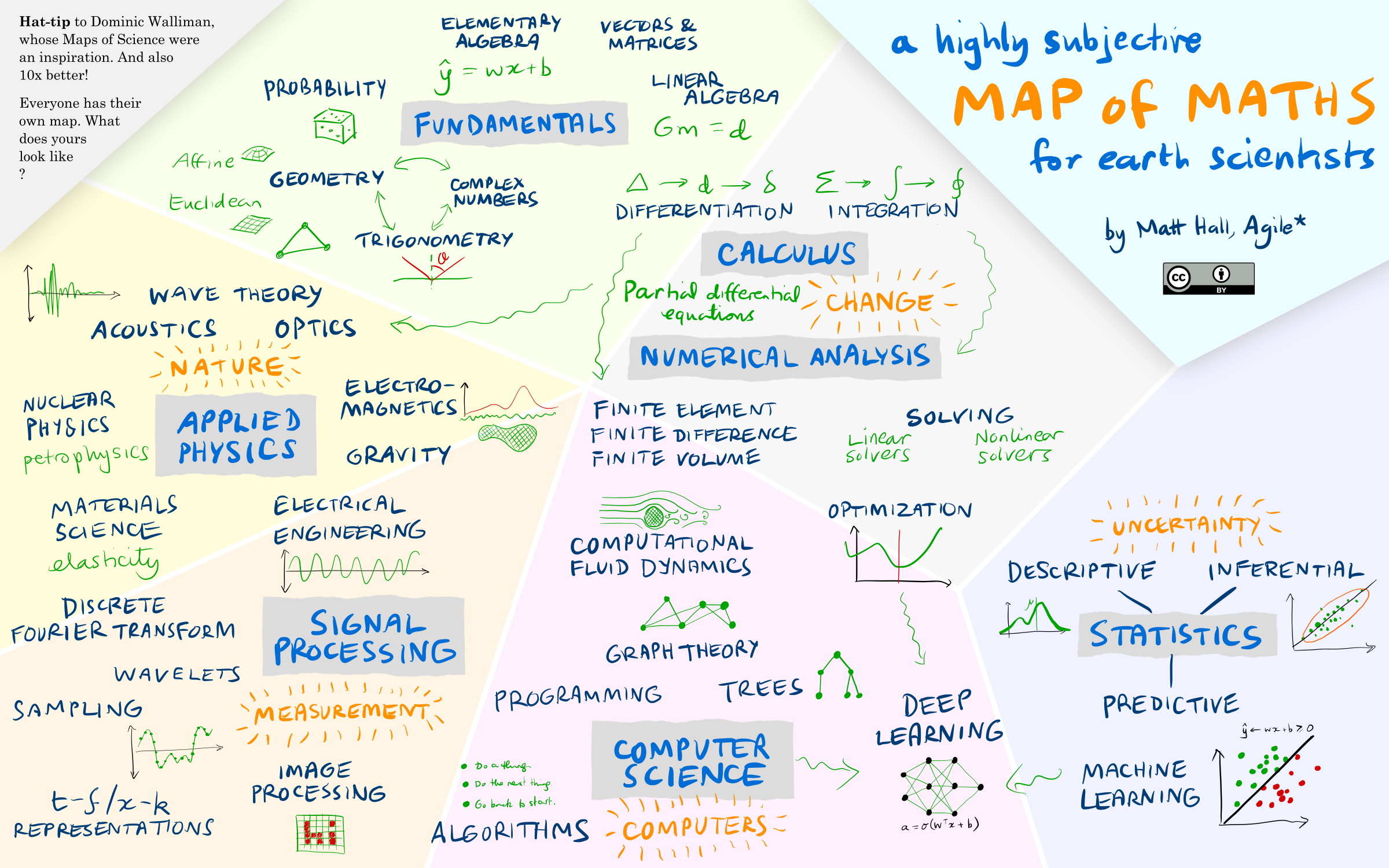
It was fun to draw, but I highly doubt that it’s any practical use. The conclusion I came to is: there is no path. In fact, this artificially flattened projection of the n-dimensional mathiverse — no doubt reflecting my own weak grasp on half of these topics — is probably a unique, personal perspective. It reflects my interests and my nonlinear journey from A-level calculus (which I loved) to undergraduate maths (which I found very hard) to… whatever half-truths I know today.

But I want to learn, where do I start?

So if there is no path, what can you do to improve? Where should you start? How can you learn? Easy: follow your nose. Start with a project — something that interests you, something you’ll stick with. Maybe it’s a spreadsheet you have, or a plot you want to make. When you get to the maths, as you inevitably will, dig in. Read around. Google things. Get a whiteboard.

As an example, when I worked on the tricky (and unsolved!) task of recovering data from pseudocolour images, my maths journey looked something like this:

Images ➡ clustering ➡ RGB vectors ➡ distance metrics ➡ k-d trees ➡ graphs ➡ Hamiltonian paths ➡ TSP solvers

Admittedly, there’s some computer science in there too, but hey, this is applied maths.

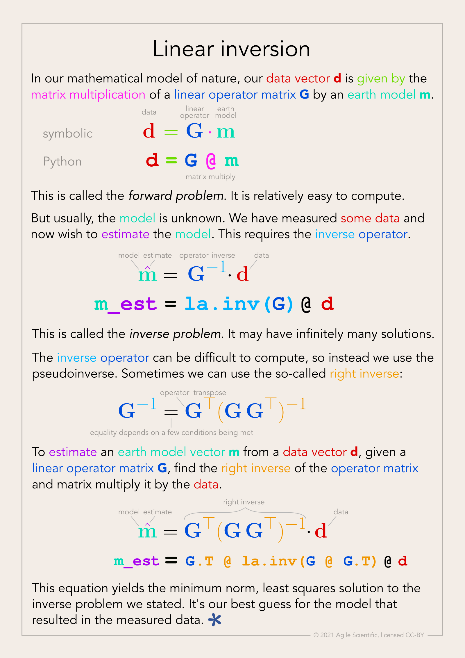
As I described recently in Illuminated equations, there are several ways to serve, and consume, mathematical ideas: words, pictures, plots, symbols, annotations, and code (and probably some others). Seek out sources that give you three or more of these things. For me, being able to run some code makes a huge difference. Indeed, learning Python has directly led to me reading entire books on graph theory, linear algebra, deep learning, Fourier transforms, and all sorts of other things.

Well, learning Python and watching Numberphile.

I think it’s a myth that you have to be good at maths to learn to code. Instead, I think learning to code can — if you want — help make you good, or at least better, at maths. By giving you a way to try things without fully knowing what you are doing (after all, np.fft.fft(x) is pretty easy to type!), code gives you a way to peek at the answer. If you do it often enough, and follow up with some reading, understanding follows eventually.

Illuminated equations

Last year I wrote a post about annotated equations, and why they are useful teaching tools. But I never shared all the cool examples people tweeted back, and some of them are too good not to share.

Let’s start with this one from Andrew Alexander that he uses to explain complex number notation:

Paige Bailey tweeted some examples of annotated equations and code from the reinforcement learning tutorial, Building a Powerful DQN in TensorFlow by Sebastian Theiler. Here’s one of the algorithms, with slightly muted annotations:

Finally, Jesper Dramsch shared a new one today (and reminded me that I never finished this post). It links to Edward Raff’s book, Inside Deep Learning, which has some nice annotations, e.g. expressing a fundamental idea of machine learning:

---

Dynamic explication

The annotations are nice, but it’s quite hard to fully explain an equation or algorithm in one shot like this. It’s easier to do, and easier to digest, over time, in a presentation. I remember a wonderful presentation by Ross Mitchell (then U of Calgary) at the also brilliant lunchtime mathematics lectures that Shell used to sponsor in Calgary. He unpeeled time-frequency analysis, especially the S transform, and I still think about his talk today.

What Ross understood is that the learner really wants to see the maths build, more or less from first principles. Here’s a nice example — admittedly in the non-ideal medium of Twitter: make sure you read the whole thread — from Darrel Francis, a cardiologist at Imperial Colege, London:

I've realised that some highly educated people find formulae like this difficult to understand. pic.twitter.com/QZcs55VMTO

— Prof Darrel Francis ☺ Mk CardioFellows Great Again (@ProfDFrancis) April 15, 2020

A video is even more dynamic of course. Josef Murad shared a video in which he derives the Navier–Stokes equation:

In this video, Grant Sanderson, perhaps the equation explainer nonpareil, unpacks the Fourier transform. He creeps up on the equation, starting instead with building the intuition around frequency decomposition:

If you’d like to try making this sort of thing, you might like to know that Sanderson’s Python software, manim, is open source.

---

Multi-modal explication

Sanderson illustrates nicely that the teacher has several pedagogic tools at their disposal:

• The spoken word.

• The written word, especially the paragraph describing a function.

• A symbolic representation of the function.

• A graphical representation of the function.

• A code representation of the function, which might also have a docstring, which is a formal description of the code, its inputs, and its outputs. It might also produce the graphical representation.

• Still other modes, e.g. pseudocode (see Theiler’s example, above), a cartoon (esssentially a ‘pseudofigure’),

Virtually all of these things are, or can be dynamic (in a video, on a whiteboard) and annotated. They approach the problem from different directions. The spoken and written descriptions should be rigorous and unambiguous, but this can make them clumsy. Symbolic maths can be useful to those that can read it, but authors must take care to define symbols properly and to be consistent. The code representation must be strict (assuming it works), but might be hard for non-programmers to parse. Figures help most people, but are more about building intuition than providing the detail you might need for implementation, say. So perhaps the best explanations have several modes of explication.

In this vein of multi-modal explication, Jeremy Howard shared a nice example from his book, Deep learning for coders, of combining text, symbolic maths, and code:

Eventually I settled on calling these things, that go beyond mere annotation, illuminated equations (not to directly compare them to the beautiful works of devotion produced by monks in the 13th century, but that’s the general idea). I made an attempt to describe linear regression and the neural network equation (not sure what else to call it!) in a series of tweets last year. Here’s the all-in-one poster version (as a PDF):

---

There’s nothing intuitive about physics, maths, or programming. The more tricks we have for spreading intuition about these important scientific tools, the better. I think there’s something in illuminated equations for teachers to practice — and students too. In fact, Jackie Caplan-Auerbach decribes coaching her students in creating ‘equation dictionaries’ in her geophysics classes. I think this is a wonderful idea.

If you’re teaching or learning maths, I’d love to hear your thoughts. Are these things worth the effort to produce? Do you have any favourite examples to share?

Visual explanations of mathematics

It is thought that Euclid wrote Elements in about 300 BC, but Oliver Byrne turned it into one of the true gems of visualization — and made it about 100 times more readable. By seamlessly combining typeset text (Caslon, if you’re interested) with minimalist geometric drawings in primary colours, he didn’t just reproduce the text; he explained it in a new way.

If you like the look of it, it’s even cooler in Nicholas Rougeur’s beautiful interactive version.

This is a classic example of what Edward Tufte, the modern saint of visualization, calls a visual explanation (he wrote a whole book about the subject). We’ve written about the subject before (for example, see Evan’s 2014 post, Graphics that repay careful study). Figures and charts should do more than merely illustrate, they should elucidate.

Too often, equations — for example the myriad equations in any volume of GEOPHYSICS — do not elucidate. Indeed, they barely even illustrate. In some cases, it’s worse: they obfuscate. You might think mathematics is too dry, or too steeped in convention, for it to be any other way. Equations just are. But Byrne showed us that we can do better.

A few years ago, in an attempt to broaden my geophysical knowledge, I bought a copy of Daniel Fleisch’s book on Maxwell’s equations. It’s excellent, and the others in the series are good too. I especially liked the annotated equations; I’ve lightened the annotations in this version, to put them on a separate visual ‘layer’:

In 2010, Randall Munroe of xkcd applied a similar strategy to label The Flake Equation, his parody of the Drake equation:

There are still other examples out there.

Later, I came across some lovely colourized equations by Stuart Riffle, a game developer. There was a bit of buzz about them on social media. Most people loved them, but a few pointed out that they suffer from the ‘legend lookup’ problem, and the colours he chose might not be great for colourblind people. Still, I like the concept — here’s the Fourier transform:

Direct annotation, something Tufte always advocates, avoids the legend lookup problem. In his 2016 Geophysics Tutorial on finite volume methods, Rowan Cockett showed that colour and labels can work together:

And in his Observable post on the predator–prey interaction, modern visualization legend Mike Bostock avoids the problem entirely with the use of pictograms: direct representation of what the symbols represent:

Observable is interesting because the documents are runnable code. And this reminds us that mathematics — equations, data structures, and so on — has another expression: code. While symbolic representation speaks directly to some people, code speaks to others, probably more. Look at Randall Munroe’s annotation of a Wolfram Alpha equation (similar to an Excel formula) from his (wonderful) book, What If:

What I love about this is the direct path to exploring the function yourself. It would take me an hour to implement Fleisch’s electric field integral in code, even with the annotations. Typing in this — admittedly less useful — rocket golf equation will take me two minutes. Expressing mathematics in code is the ultimate explicit and practical expression of an idea.

We have lots of tools to write better mathematics: LaTeX, markdown, Jupyter Notebooks, and so on. But it feels like nothing has really converged yet. Technology that seamlessly mixes symbolic equations, illustrative-and-explicative annotation, and runnable code is, I am sure, not far off. Until then, we do the best we can with the tools we have.

---

Have you seen nice examples of annotated equations? I’d love to hear about them; let me know in the comments!

---

Don’t miss the follow-up post from 2021: Illuminated equations.

---

The work by Byrne is out of copyright. Those by Munroe and Cockett are openly licensed under Creative Commons. The work of Fleisch and Bostock are used in accordance with Fair Use doctrine.

Real and apparent seismic frequency

There's a Jupyter Notebook for you to follow along with this tutorial. You can run it right here in your browser.

---

We often use Ricker wavelets to model seismic, for example when making a synthetic seismogram with which to help tie a well. One simple way to guesstimate the peak or central frequency of the wavelet that will model a particlar seismic section is to count the peaks per unit time in the seismic. But this tends to overestimate the actual frequency because the maximum frequency of a Ricker wavelet is more than the peak frequency. The question is, how much more?

To investigate, let's make a Ricker wavelet and see what it looks like in the time and frequency domains.

>>> T, dt, f = 0.256, 0.001, 25

>>> import bruges
>>> w, t = bruges.filters.ricker(T, dt, f, return_t=True)

>>> import scipy.signal
>>> f_W, W = scipy.signal.welch(w, fs=1/dt, nperseg=256)

When we count the peaks in a section, the assumption is that this apparent frequency — that is, the reciprocal of apparent period or distance between the extrema — tells us the dominant or peak frequency.

To help see why this assumption is wrong, let's compare the Ricker with a signal whose apparent frequency does match its peak frequency: a pure cosine:

>>> c = np.cos(2 * 25 * np.pi * t)
>>> f_C, C = scipy.signal.welch(c, fs=1/dt, nperseg=256)

Notice that the signal is much narrower in bandwidth. If we allowed more oscillations, it would be even narrower. If it lasted forever, it would be a spike in the frequency domain.

Let's overlay the signals to get a picture of the difference in the relative periods:

The practical consequence of this is that if we estimate the peak frequency to be \(f\ \mathrm{Hz}\), then we need to reduce \(f\) by some factor if we want to design a wavelet to match the data. To get this factor, we need to know the apparent period of the Ricker function, as given by the time difference between the two minima.

Let's look at a couple of different ways to find those minima: numerically and analytically.

Find minima numerically

We'll use scipy.optimize.minimize to find a numerical solution. In order to use it, we'll need a slightly different expression for the Ricker function — casting it in terms of a time basis t. We'll also keep f as a variable, rather than hard-coding it in the expression, to give us the flexibility of computing the minima for different values of f.

Here's the equation we're implementing:

$$ w(t, f) = (1 - 2\pi^2 f^2 t^2)\ e^{-\pi^2 f^2 t^2} $$

In Python:

>>> def ricker(t, f):
>>>     return (1 - 2*(np.pi*f*t)**2) * np.exp(-(np.pi*f*t)**2)

Check that the wavelet looks like it did before, by comparing the output of this function when f is 25 with the wavelet w we were using before:

>>> f = 25
>>> np.allclose(w, ricker(t, f=25))
True

Now we call SciPy's minimize function on our ricker function. It itertively searches for a minimum solution, then gives us the x (which is really t in our case) at that minimum:

>>> import scipy.optimize
>>> f = 25
>>> scipy.optimize.minimize(ricker, x0=0, args=(f))

fun: -0.4462603202963996
 hess_inv: array([[1]])
      jac: array([-2.19792128e-07])
  message: 'Optimization terminated successfully.'
     nfev: 30
      nit: 1
     njev: 10
   status: 0
  success: True
        x: array([0.01559393])

So the minimum amplitude, given by fun, is -0.44626 and it occurs at an x (time) of \(\pm 0.01559\ \mathrm{s}\).

In comparison, the minima of the cosine function occur at a time of \(\pm 0.02\ \mathrm{s}\). In other words, the period appears to be \(0.02 - 0.01559 = 0.00441\ \mathrm{s}\) shorter than the pure waveform, which is...

>>> (0.02 - 0.01559) / 0.02
0.22050000000000003

...about 22% shorter. This means that if we naively estimate frequency by counting peaks or zero crossings, we'll tend to overestimate the peak frequency of the wavelet by about 22% — assuming it is approximately Ricker-like; if it isn't we can use the same method to estimate the error for other functions.

This is good to know, but it would be interesting to know if this parameter depends on frequency, and also to have a more precise way to describe it than a decimal. To get at these questions, we need an analytic solution.

Find minima analytically

Python's SymPy package is a bit like Maple — it understands math symbolically. We'll use sympy.solve to find an analytic solution. It turns out that it needs the Ricker function writing in yet another way, using SymPy symbols and expressions for \(\mathrm{e}\) and \(\pi\).

import sympy as sp
t, f = sp.Symbol('t'), sp.Symbol('f')
r = (1 - 2*(sp.pi*f*t)**2) * sp.exp(-(sp.pi*f*t)**2)

Now we can easily find the solutions to the Ricker equation, that is, the times at which the function is equal to zero:

>>> sp.solvers.solve(r, t)
[-sqrt(2)/(2*pi*f), sqrt(2)/(2*pi*f)]

But this is not quite what we want. We need the minima, not the zero-crossings.

Maybe there's a better way to do this, but here's one way. Note that the gradient (slope or derivative) of the Ricker function is zero at the minima, so let's just solve the first time derivative of the Ricker function. That will give us the three times at which the function has a gradient of zero.

>>> dwdt = sp.diff(r, t)
>>> sp.solvers.solve(dwdt, t)
[0, -sqrt(6)/(2*pi*f), sqrt(6)/(2*pi*f)]

In other words, the non-zero minima of the Ricker function are at:

$$ \pm \frac{\sqrt{6}}{2\pi f} $$

Let's just check that this evaluates to the same answer we got from scipy.optimize, which was 0.01559.

>>> np.sqrt(6) / (2 * np.pi * 25)
0.015593936024673521

The solutions agree.

While we're looking at this, we can also compute the analytic solution to the amplitude of the minima, which SciPy calculated as -0.446. We just plug one of the expressions for the minimum time into the expression for r:

>>> r.subs({t: sp.sqrt(6)/(2*sp.pi*f)})
-2*exp(-3/2)

Apparent frequency

So what's the result of all this? What's the correction we need to make?

The minima of the Ricker wavelet are \(\sqrt{6}\ /\ \pi f_\mathrm{actual}\ \mathrm{s}\) apart — this is the apparent period. If we're assuming a pure tone, this period corresponds to an apparent frequency of \(\pi f_\mathrm{actual}\ /\ \sqrt{6}\ \mathrm{Hz}\). For \(f = 25\ \mathrm{Hz}\), this apparent frequency is:

>>> (np.pi * 25) / np.sqrt(6)
32.06374575404661

If we were to try to model the data with a Ricker of 32 Hz, the frequency will be too high. We need to multiply the frequency by a factor of \(\sqrt{6} / \pi\), like so:

>>> 32.064 * np.sqrt(6) / (np.pi)
25.00019823475659

This gives the correct frequency of 25 Hz.

To sum up, rearranging the expression above:

$$ f_\mathrm{actual} = f_\mathrm{apparent} \frac{\sqrt{6}}{\pi} $$

Expressed as a decimal, the factor we were seeking is therefore \(\sqrt{6}\ /\ \pi\):

>>> np.sqrt(6) / np.pi
0.779696801233676

That is, the reduction factor is 22%.

---

Curious coincidence: in the recent Pi Day post, I mentioned the Riemann zeta function of 2 as a way to compute \(\pi\). It evaluates to \((\pi / \sqrt{6})^2\). Is there a million-dollar connection between the humble Ricker wavelet and the Riemann hypothesis?

I doubt it.

Happy π day, Einstein

It's Pi Day today, and also Einstein's 139th birthday. MIT celebrates it at 6:28 pm — in honour of pi's arch enemy, tau — by sending out its admission notices.

And Stephen Hawking died today. He will leave a great, black hole in modern science. I saw him lecture in London not long after A Brief History of Time came out. It was one of the events that inspired me along my path to science. I recall he got more laughs than a lot of stand-ups I've seen.

But I can't really get behind 3/14. The weird American way of writing dates, mixed-endian style, really irks me. As a result, I have previously boycotted Pi Day, instead celebrating it on 31/4, aka 31 April, aka 1 May. Admittedly, this takes the edge off the whole experience a bit, so I've decided to go full big-endian and adopt ISO-8601 from now on, which means Pi Day is on 3141-5-9. Expect an epic blog post that day.

Transcendence

Anyway, I will transcend the bickering over dates (pausing only to reject 22/7 and 6/28 entirely so don't even start) to get back to pi. It so happens that Pi Day is of great interest in our house this year because my middle child, Evie (10), is a bit obsessed with pi at the moment. Obsessed enough to be writing a book about it (she writes a lot of books; some previous topics: zebras, Switzerland, octopuses, and Settlers of Catan fan fiction, if that's even a thing).

I helped her find some ways to generate pi numerically. My favourite one uses Riemann's zeta function, which we'd recently watched a Numberphile video about. It's the sum of the reciprocals of the natural numbers raised to increasing powers:

$$\zeta(s) = \sum_{n=1}^\infty \frac{1}{n^s}$$

Leonhard Euler solved the Basel problem in 1734, proving that \(\zeta(2) = \pi^2 / 6\), so you can compute pi slowly with a naive implementation of the zeta function:

def zeta(s, terms=1000):
    z = 0
    for t in range(1, int(terms)):
        z += 1 / t**s
    return z

(6 * zeta(2, terms=1e7))**0.5

Which returns pi, correct to 6 places:

3.141592558095893

Or you can use one of the various optimized versions of the zeta function, for example this one from the floating point math library mpmath (which I got from this awesome list of 100 ways to compute pi):

>>> from mpmath import *
>>> mp.dps = 50
>>> mp.pretty = True
>>>
>>> sqrt(6*zeta(2))
3.1415926535897932384626433832795028841971693993751068

...which is correct to 50 decimal places.

Here's the bit of Evie's book where she explains a bit about transcendental numbers.

Evie's book shows the relationships between the sets of natural numbers (N), integers (Z), rationals (Q), algebraic numbers (A), and real numbers (R). Transcendental numbers are real, but not algebraic. (Some definitions also let them be complex.)

I was interested in this, because while I 'knew' that pi is transcendental, I couldn't really articulate what that really meant, and why (say) √2, which is also irrational, is not also transcendental. Succinctly, transcendental means 'non-algebraic' (equivalent to being non-constructible). Since √2 is obviously the solution to \(x^2 - 2 = 0\), it is algebraic and therefore not transcendental. 

Weirdly, although hardly any numbers are known to be transcendental, almost all real numbers are. Isn't maths awesome?

Have a transcendental pi day!

---

The xkcd comic is by Randall Munroe and licensed CC-BY-NC.

Jounce, Crackle and Pop

I saw this T-shirt recently, and didn't get it. (The joke or the T-shirt.)

It turns out that the third derivative of displacement \(x\) with respect to time \(t\) — that is, the derivative of acceleration \(\mathbf{a}\) — is called 'jerk' (or sometimes, boringly, jolt, surge, or lurch) and is measured in units of m/s³. 

So far, so hilarious, but is it useful? It turns out that it is. Since the force \(\mathbf{F}\) on a mass \(m\) is given by \(\mathbf{F} = m\mathbf{a}\), you can think of jerk as being equivalent to a change in force. The lurch you feel at the onset of a car's acceleration — that's jerk. The designers of transport systems and rollercoasters manage it daily.

$$ \mathrm{jerk,}\ \mathbf{j} = \frac{\mathrm{d}^3 x}{\mathrm{d}t^3}$$

Here's a visualization of velocity (green line) of a Tesla Model S driving in a parking lot. The coloured stripes show the acceleration (upper plot) and the jerk (lower plot). Notice that the peaks in jerk correspond to changes in acceleration.

The snap you feel at the start of the lurch? That's jounce  — the fourth derivative of displacement and the derivative of jerk. Eager et al (2016) wrote up a nice analysis of these quantities for the examples of a trampolinist and roller coaster passenger. Jounce is sometimes called snap... and the next two derivatives are called crackle and pop. 

What about momentum?

If the momentum \(\mathrm{p}\) of a mass \(m\) moving at a velocity \(v\) is \(m\mathbf{v}\) and \(\mathbf{F} = m\mathbf{a}\), what is mass times jerk? According to the physicist Philip Gibbs, who investigated the matter in 1996, it's called yank:

“Momentum equals mass times velocity.
Force equals mass times acceleration.
Yank equals mass times jerk.
Tug equals mass times snap.
Snatch equals mass times crackle.
Shake equals mass times pop.”

There are jokes in there, help yourself.

What about integrating?

Clearly the integral of jerk is acceleration, and that of acceleration is velocity, the integral of which is displacement. But what is the integral of displacement with respect to time? It's called absement, and it's a pretty peculiar quantity to think about. In the same way that an object with linearly increasing displacement has constant velocity and zero acceleration, an object with linearly increasing absement has constant displacement and zero velocity. (Constant absement at zero displacement gives rise to the name 'absement': an absence of displacement.)

Integrating displacement over time might be useful: the area under the displacement curve for a throttle lever could conceivably be proportional to fuel consumption for example. So absement seems to be a potentially useful quantity, measured in metre-seconds.

Integrate absement and you get absity (a play on 'velocity'). Keep going and you get abseleration, abserk, and absounce. Are these useful quantities? I don't think so. A quick look at them all — for the same Tesla S dataset I used before — shows that the loss of detail from multiple cumulative summations makes for rather uninformative transformations: 

---

You can reproduce the figures in this article with the Jupyter Notebook Jerk_jounce_etc.ipynb. Or you can launch a Binder right here in your browser and play with it there, without installing a thing!

---

References

David Eager et al (2016). Beyond velocity and acceleration: jerk, snap and higher derivatives. Eur. J. Phys. 37 065008. DOI: 10.1088/0143-0807/37/6/065008

Amarashiki (2012). Derivatives of position. The Spectrum of Riemannium blog, retrieved on 4 Mar 2018.

The dataset is from Jerry Jongerius's blog post, The Tesla (Elon Musk) and
New York Times (John Broder) Feud. I have no interest in the 'feud', I just wanted a dataset.

The T-shirt is from Chummy Tees; the image is their copyright and used here under Fair Use terms.

The vintage Snap, Crackle and Pop logo is copyright of Kellogg's and used here under Fair Use terms.

The norm and simple solutions

Last time I wrote about different ways of calculating distance in a vector space — say, a two-dimensional Euclidean plane like the streets of Portland, Oregon. I showed three ways to reckon the distance, or norm, between two points (i.e. vectors). As a reminder, using the distance between points u and v on the map below this time:

$$ \|\mathbf{u} - \mathbf{v}\|_1 = |u_x - v_x| + |u_y - v_y| $$

$$ \|\mathbf{u} - \mathbf{v}\|_2 = \sqrt{(u_x - v_x)^2 + (u_y - v_y)^2} $$

$$ \|\mathbf{u} - \mathbf{v}\|_\infty = \mathrm{max}(|u_x - v_x|, |u_y - v_y|) $$

Let's think about all the other points on Portland's streets that are the same distance away from u as v is. Again, we have to think about what we mean by distance. If we're walking, or taking a cab, we'll need to think about \(\ell_1\) — the sum of the distances in x and y. This is shown on the left-most map, below.

View fullsize

For simplicity, imagine u is the origin, or (0, 0) in Cartesian coordinates. Then v is (0, 4). The sum of the distances is 4. Looking for points with the same sum, we find the pink points on the map.

If we're thinking about how the crow flies, or \(\ell_2\) norm, then the middle map sums up the situation: the pink points are all equidistant from u. All good: this is what we usually think of as 'distance'.

The \(\ell_\infty\) norm, on the other hand, only cares about the maximum distance in any direction, or the maximum element in the vector. So all points whose maximum coordinate is 4 meet the criterion: (1, 4), (2, 4), (4, 3) and (4, 0) all work.

You might remember there was also a weird definition for the \(\ell_0\) norm, which basically just counts the non-zero elements of the vector. So, again treating u as the origin for simplicity, we're looking for all the points that, like v, have only one non-zero Cartesian coordinate. These points form an upright cross, like a + sign (right).

So there you have it: four ways to draw a circle.

Wait, what?

A circle is just a set of points that are equidistant from the centre. So, depending on how you define distance, the shapes above are all 'circles'. In particular, if we normalize the (u, v) distance as 1, we have the following unit circles:

View fullsize

It turns out we can define any number of norms (if you like the sound of \(\ell_{2.4}\) or \(\ell_{240}\) or \(\ell_{0.024}\)...) but most of the time, these will suffice. You can probably imagine the shapes of the unit circles defined by these other norms.

What can we do with this stuff?

Let's think about solving equations. Think about solving this:

$$ x + 2y = 8 $$

I'm sure you can come up with a soluiton in your head, x = 6 and y = 1 maybe. But one equation and two unknowns means that this problem is underdetermined, and consequently has an infinite number of solutions. The solutions can be visualized geometrically as a line in the Euclidean plane (right).

But let's say I don't want solutions like (3.141590, 2.429205) or (2742, –1367). Let's say I want the simplest solution. What's the simplest solution?

This is a reasonable question, but how we answer it depends how we define 'simple'. One way is to ask for the nearest solution to the origin. Also reasonable... but remember that we have a few different ways to define 'nearest'. Let's start with the everyday definition: the shortest crow-flies distance from the origin. The crow-flies, \(\ell_2\) distances all lie on a circle, so you can imagine starting with a tiny circle at the origin, and 'inflating' it until it touches the line \(x + 2y - 8 = 0\). This is usually called the minimum norm solution, minimized on \(\ell_2\). We can find it in Python like so:

    import numpy.linalg as la
    A = [[1, 2]]
    b = [8]
    la.lstsq(A, b)

The result is the vector (1.6, 3.2). You could almost have worked that out in your head, but imagine having 1000 equations to solve and you start to appreciate numpy.linalg. Admittedly, it's even easier in Octave (or MATLAB if you must) and Julia:

    A = [1 2]
    b = [8]
    A \ b

But remember we have lots of norms. It turns out that minimizing other norms can be really useful. For example, minimizing the \(\ell_1\) norm — growing a diamond out from the origin — results in (0, 4). The \(\ell_0\) norm gives the same sparse* result. Minimizing the \(\ell_\infty\) norm leads to \( x = y = 8/3 \approx 2.67\).

This was the diagram I wanted to get to when I started with the 'how far away is the supermarket' business. So I think I'll stop now... have fun with Norm!

---

* I won't get into sparsity now, but it's a big deal. People doing big computations are always looking for sparse representations of things. They use less memory, are less expensive to compute with, and are conceptually 'neater'. Sparsity is really important in compressed sensing, which has been a bit of a buzzword in geophysics lately.

The norm: kings, crows and taxicabs

How far away is the supermarket from your house? There are lots of ways of answering this question:

• As the crow flies. This is the green line from \(\mathbf{a}\) to \(\mathbf{b}\) on the map below.

• The 'city block' driving distance. If you live on a grid of streets, all possible routes are the same length — represented by the orange lines on the map below.

• In time, not distance. This is usually a more useful answer... but not one we're going to discuss today.

Don't worry about the mathematical notation on this map just yet. The point is that there's more than one way to think about the distance between two points, or indeed any measure of 'size'.

Higher dimensions

The map is obviously two-dimensional, but it's fairly easy to conceive of 'size' in any number of dimensions. This is important, because we often deal with more than the 2 dimensions on a map, or even the 3 dimensions of a seismic stack. For example, we think of raw so-called 3D seismic data as having 5 dimensions (x position, y position, offset, time, and azimuth). We might even formulate a machine learning task with a hundred or more dimensions (or 'features').

Why do we care about measuring distances in high dimensions? When we're dealing with data in these high-dimensional spaces, 'distance' is a useful way to measure the similarity between two points. For example, I might want to select those samples that are close to a particular point of interest. Or, from among the points satisfying some constraint, select the one that's closest to the origin.

Definitions and nomenclature

We'll define norms in the context of linear algebra, which is the study of vector spaces (think of multi-dimensional 'data spaces' like the 5D space of seismic data). A norm is a function that assigns a positive scalar size to a vector \(\mathbf{v}\) , with a size of zero reserved for the zero vector (in the Cartesian plane, the zero vector has coordinates (0, 0) and is usually called the origin). Any norm \(\|\mathbf{v}\|\) of this vector satisfies the following conditions:

1. Absolutely homogenous. The norm of \(\alpha\mathbf{v}\) is equal to \(|\alpha|\) times the norm of \(\mathbf{v}\).

2. Subadditive. The norm of \( (\mathbf{u} + \mathbf{v}) \) is less than or equal to the norm of \(\mathbf{u}\) plus the norm of \(\mathbf{v}\). In other words, the norm satisfies the triangle inequality.

3. Positive. The first two conditions imply that the norm is non-negative.

4. Definite. Only the zero vector has a norm of 0.

Kings, crows and taxicabs

Let's return to the point about lots of ways to define distance. We'll start with the most familiar definition of distance on a map— the Euclidean distance, aka the \(\ell_2\) or \(L_2\) norm (confusingly, sometimes the two is written as a superscript), the 2-norm, or sometimes just 'the norm' (who says maths has too much jargon?). This is the 'as-the-crow-flies distance' on the map above, and we can calculate it using Pythagoras:

$$ \|\mathbf{v}\|_2 = \sqrt{(a_x - b_x)^2 + (a_y - b_y)^2} $$

You can extend this to an arbitrary number of dimensions, just keep adding the squared elementwise differences. We can also calculate the norm of a single vector in n-space, which is really just the distance between the origin and the vector:

$$ \|\mathbf{u}\|_2 = \sqrt{u_1^2 + u_2^2 + \ldots + u_n^2}  = \sqrt{\mathbf{u} \cdot \mathbf{u}} $$

As shown here, the 2-norm of a vector is the square root of its dot product with itself.

So the crow-flies distance is fairly intuitive... what about that awkward city block distance? This is usually referred to as the Manhattan distance, the taxicab distance, the \(\ell_1\) or \(L_1\) norm, or the 1-norm. As you can see on the map, it's just the sum of the absolute distances in each dimension, x and y in our case:

$$ \|\mathbf{v}\|_1 = |a_x - b_x| + |a_y - b_y| $$

What's this magic number 1 all about? It turns out that the distance metric can be generalized as the so-called p-norm, where p can take any positive value up to infinity. The definition of the p-norm is consistent with the two norms we just met:

$$ \| \mathbf{u} \|_p = \left( \sum_{i=1}^n | u_i | ^p \right)^{1/p} $$

[EDIT, May 2021: This generalized version is sometimes called the Minkowski distance, e.g. in the scipy documentation.]

In practice, I've only ever seen p = 1, 2, or infinity (and 0, but we'll get to that). Let's look at the meaning of the \(\infty\)-norm, aka the \(\ell_\infty\) or \(L_\infty\) norm, which is sometimes called the Chebyshev distance or chessboard distance (because it defines the minimum number of moves for a king to any given square):

$$ \|\mathbf{v}\|_\infty = \mathrm{max}(|a_x - b_x|, |a_y - b_y|) $$

In other words, the Chebyshev distance is simply the maximum element in a given vector. In a nutshell, the infinitieth root of the sum of a bunch of numbers raised to the infinitieth power, is the same as the infinitieth root of the largest of those numbers raised to the infinitieth power — because infinity is weird like that.

What about p = 0?

Infinity is weird, but so is zero sometimes. Taking the zeroeth root of a lot of ones doesn't make a lot of sense, so mathematicians often redefine the \(\ell_0\) or \(L_0\) "norm" (not a true norm) as a simple count of the number of non-zero elements in a vector. In other words, we toss out the 0th root, define \(0^0 := 0 \) and do:

$$ \| \mathbf{u} \|_0 = |u_1|^0 + |u_2|^0 + \cdots + |u_n|^0 $$

(Or, if we're thinking about the points \(\mathbf{a}\) and \(\mathbf{b}\) again, just remember that \(\mathbf{v}\) = \(\mathbf{a}\) - \(\mathbf{b}\).)

Computing norms

Let's take a quick look at computing the norm of some vectors in Python:

>>> import numpy as np

>>> a = np.array([1, 1]).T
>>> b = np.array([6, 5]).T

>>> L_0 = np.count_nonzero(a - b)
2

>>> L_1 = np.sum(np.abs(a - b))
9

>>> L_2 = np.sqrt((a - b) @ (a - b))
6.4031242374328485

>>> L_inf = np.max(np.abs(a - b))
5

>>> # Using NumPy's `linalg` module:
>>> import numpy.linalg as la
>>> for p in (0, 1, 2, np.inf):
>>>    print("L_{} norm = {}".format(p, la.norm(a - b, p)))
L_0 norm = 2.0
L_1 norm = 9.0
L_2 norm = 6.4031242374328485
L_inf norm = 5.0

What can we do with all this?

So far, so good. But what's the point of these metrics? How can we use them to solve problems? We'll get into that in a future post, so don't go too far!

For now I'll leave you to play with this little interactive demo of the effect of changing p-norms on a Voronoi triangle tiling — it's by Sarah Greer, a geophysics student at UT Austin. 

---

UPDATE — The next post is The norm and simple solutions, which looks at how these different norms can be used to solve real-world problems.

The quick green forsterite jumped over the lazy dolomite

The best-known pangram — a sentence containing every letter of the alphabet —  is probably

“The quick brown fox jumped over the lazy dog.”

There are lots of others of course. If you write like James Joyce, there are probably an infinite number of others. The point is to be short, and one of the shortest, with only 29 letters (!), even has a geological flavour:

“Sphinx of black quartz, judge my vow.”

I know what you're thinking: Cool, but what's the shortest set of mineral names that uses all the letters of the alphabet? What logophiliac geologist would not wonder the same thing?

Well, we posed this question in the most recent "Riddle me this" segment on the Undersampled Radio podcast. This blog post is my solution.

---

The set cover problem

Finding pangrams in a list of words amounts to solving the classical set cover problem:

“Given a set of elements \(\{U_1, U_2,\ldots , U_n\}\) (called the ‘universe’) and a collection \(S\) of \(m\) sets whose union equals the universe, the set cover problem is to identify the smallest sub-collection of \(S\) whose union equals (or ‘covers’) the universe.”

Our universe is the alphabet, and our \(S\) is the list of \(m\) mineral names. There is a slight twist in our case: the set cover problem wants the smallest subset of \(S\) — the fewest members. But in this problem, I suspect there are several 4-word solutions (judging from my experiments), so I want the smallest total size of the members of the subset. That is, I want the fewest total letters in the solution.

The solution

The set cover problem was shown to be NP-complete in 1972. What does this mean? It means that it's easy to tell if you have an answer (do you have all the letters of the alphabet?), but the only way to arrive at a solution is — to oversimplify massively — by brute force. (If you're interested in this stuff, this edition of the BBC's In Our Time is one of the best intros to P vs NP and complexity theory that I know of.)

Anyway, the point is that if we find a better way than brute force to solve this problem, then we need to write a paper about it immediately, claim our prize, collect our turkey, then move to a sunny tax haven with good water and double-digit elevation.

So, this could take a while: there are over 95 billion ways to draw 3 words from my list of 4600 mineral names. If we need 4 minerals, there are 400 trillion combinations... and a quick calculation suggests that my laptop will take a little over 50 years to check all the combinations. 

Can't we speed it up a bit?

Brute force is one thing, but we don't need to be brutish about it. Maybe we can think of some strategies to give ourselves a decent chance:

• The list is alphabetically sorted, so randomize the list before searching. (I did this.)
• Guess some 'useful' minerals and ensure that you get to them. (I did this too, with quartz.)
• Check there are at least 26 letters in the candidate words, and (if it's only records we care about) no more than 44, because I have a solution with 45 letters (see below).
• We could sort the list into word length order. That way we search shorter things first, so we should get shorter lists (which we want) earlier.
• My solution does not depend much on Python's set type. Maybe we could do more with set theory.
• Before inspecting the last word in each list, we could make sure it contains at least one letter that's so far missing.

So far, the best solution I've come up with so far has 45 letters, so there's plenty of room for improvement:

'quartz', 'kvanefjeldite', 'abswurmbachite', 'pyroxmangite'

My solution is in this Jupyter Notebook. Please put me out of my misery by improving on it.

Great geophysicists #13: Poisson

Siméon Denis Poisson was born in Pithiviers, France, on 21 June 1781. While still a teenager, Poisson entered the prestigious École Polytechnique in Paris, and published his first papers in 1800. He was immediately befriended — or adopted, really — by Lagrange and Laplace. So it's safe to say that he got off to a pretty good start as a mathematician. The meteoric trajectory continued throughout his career, as Poisson received more or less every honour a French scientist could accumulate. Along with Laplace and Lagrange — as well as Fresnel, Coulomb, Lamé, and Fourier — his is one of the 72 names on the Eiffel Tower.

Wrong Poisson

In the first few decades following the French Revolution, which ended in 1799, France enjoyed a golden age of science. The Société d’Acrueil was a regular meeting of savants, hosted by Laplace and the chemist Claude Louis Berthollet, and dedicated to the exposition of physical phenomena. The group worked on problems like the behaviour of gases, the physics of sound and light, and the mechanics of deformable materials. Using Newton's then 120-year-old law of gravitation as an analogy, the prevailing school of thought accounted for all physical phenomena in terms of forces acting between particles. 

Poisson was not flawless. As one of the members of this intellectual inner circle, Poisson was devoted to the corpuscular theory of light. Indeed, he dismissed the wave theory of light completely, until proven wrong by Thomas Young and, most conspicuously, Augustin-Jean Fresnel. Even Poisson's ratio, the eponymous elastic modulus, wasn't the result of his dogged search for truth, but instead represents a controversy that drove the development of the three-dimensional theory of elasticity. More on this next time.

The workaholic

Although he did make time for his wife and four children — but only after 6 pm — Poisson apparently had little time for much besides mathematics. His catchphrase was

Life is only good for two things: doing mathematics and teaching it.

In the summer of 1838, he learned he had a form of tuberculosis. According to James (2002), he was unable to take time away from work for long enough to recuperate. Eventually, insisting on conducting the final exams at the Polytechnique for the 23rd year in a row, he took on more than he could handle. He died on 20 April 1840. 

---

References

Grattan-Guinness, I. (1990). Convolutions in French Mathematics, 1800-1840: From the Calculus and Mechanics to Mathematical Analysis and Mathematical Physics. Vol.1: The Setting. Springer Science & Business Media. 549 pages.

Ioan James, I (2002). Remarkable Mathematicians: From Euler to Von Neumann. Cambridge University Press, 433 pages.

The University of St Andrews MacTutor archive article on Poisson.