Real and apparent seismic frequency

There's a Jupyter Notebook for you to follow along with this tutorial. You can run it right here in your browser.


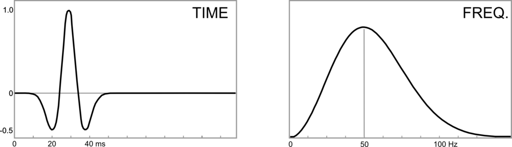
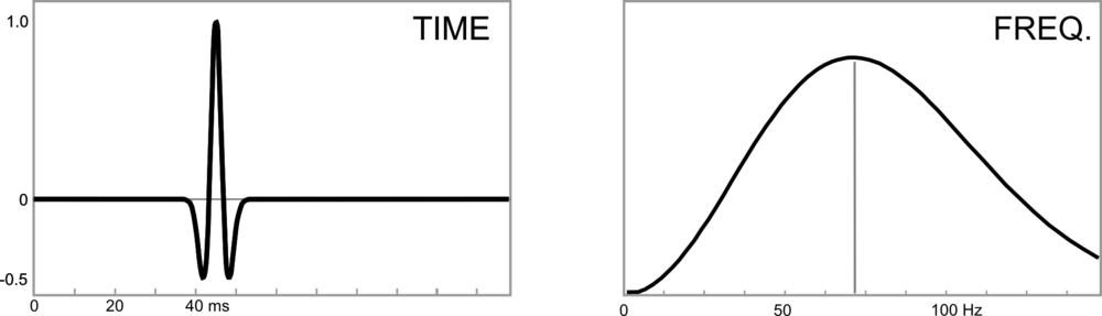
We often use Ricker wavelets to model seismic, for example when making a synthetic seismogram with which to help tie a well. One simple way to guesstimate the peak or central frequency of the wavelet that will model a particlar seismic section is to count the peaks per unit time in the seismic. But this tends to overestimate the actual frequency because the maximum frequency of a Ricker wavelet is more than the peak frequency. The question is, how much more?

To investigate, let's make a Ricker wavelet and see what it looks like in the time and frequency domains.

>>> T, dt, f = 0.256, 0.001, 25

>>> import bruges
>>> w, t = bruges.filters.ricker(T, dt, f, return_t=True)

>>> import scipy.signal
>>> f_W, W = scipy.signal.welch(w, fs=1/dt, nperseg=256)
The_frequency_of_a_Ricker_2_0.png

When we count the peaks in a section, the assumption is that this apparent frequency — that is, the reciprocal of apparent period or distance between the extrema — tells us the dominant or peak frequency.

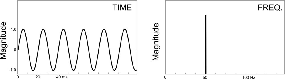
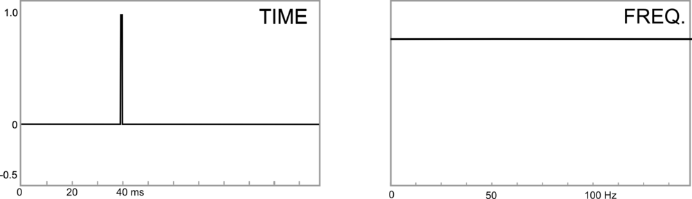
To help see why this assumption is wrong, let's compare the Ricker with a signal whose apparent frequency does match its peak frequency: a pure cosine:

>>> c = np.cos(2 * 25 * np.pi * t)
>>> f_C, C = scipy.signal.welch(c, fs=1/dt, nperseg=256)
The_frequency_of_a_Ricker_4_0.png

Notice that the signal is much narrower in bandwidth. If we allowed more oscillations, it would be even narrower. If it lasted forever, it would be a spike in the frequency domain.

Let's overlay the signals to get a picture of the difference in the relative periods:

The_frequency_of_a_Ricker_6_1.png

The practical consequence of this is that if we estimate the peak frequency to be \(f\ \mathrm{Hz}\), then we need to reduce \(f\) by some factor if we want to design a wavelet to match the data. To get this factor, we need to know the apparent period of the Ricker function, as given by the time difference between the two minima.

Let's look at a couple of different ways to find those minima: numerically and analytically.

Find minima numerically

We'll use scipy.optimize.minimize to find a numerical solution. In order to use it, we'll need a slightly different expression for the Ricker function — casting it in terms of a time basis t. We'll also keep f as a variable, rather than hard-coding it in the expression, to give us the flexibility of computing the minima for different values of f.

Here's the equation we're implementing:

$$ w(t, f) = (1 - 2\pi^2 f^2 t^2)\ e^{-\pi^2 f^2 t^2} $$

In Python:

>>> def ricker(t, f):
>>>     return (1 - 2*(np.pi*f*t)**2) * np.exp(-(np.pi*f*t)**2)

Check that the wavelet looks like it did before, by comparing the output of this function when f is 25 with the wavelet w we were using before:

>>> f = 25
>>> np.allclose(w, ricker(t, f=25))
True

Now we call SciPy's minimize function on our ricker function. It itertively searches for a minimum solution, then gives us the x (which is really t in our case) at that minimum:

>>> import scipy.optimize
>>> f = 25
>>> scipy.optimize.minimize(ricker, x0=0, args=(f))

fun: -0.4462603202963996
 hess_inv: array([[1]])
      jac: array([-2.19792128e-07])
  message: 'Optimization terminated successfully.'
     nfev: 30
      nit: 1
     njev: 10
   status: 0
  success: True
        x: array([0.01559393])

So the minimum amplitude, given by fun, is -0.44626 and it occurs at an x (time) of \(\pm 0.01559\ \mathrm{s}\).

In comparison, the minima of the cosine function occur at a time of \(\pm 0.02\ \mathrm{s}\). In other words, the period appears to be \(0.02 - 0.01559 = 0.00441\ \mathrm{s}\) shorter than the pure waveform, which is...

>>> (0.02 - 0.01559) / 0.02
0.22050000000000003

...about 22% shorter. This means that if we naively estimate frequency by counting peaks or zero crossings, we'll tend to overestimate the peak frequency of the wavelet by about 22% — assuming it is approximately Ricker-like; if it isn't we can use the same method to estimate the error for other functions.

This is good to know, but it would be interesting to know if this parameter depends on frequency, and also to have a more precise way to describe it than a decimal. To get at these questions, we need an analytic solution.

Find minima analytically

Python's SymPy package is a bit like Maple — it understands math symbolically. We'll use sympy.solve to find an analytic solution. It turns out that it needs the Ricker function writing in yet another way, using SymPy symbols and expressions for \(\mathrm{e}\) and \(\pi\).

import sympy as sp
t, f = sp.Symbol('t'), sp.Symbol('f')
r = (1 - 2*(sp.pi*f*t)**2) * sp.exp(-(sp.pi*f*t)**2)

Now we can easily find the solutions to the Ricker equation, that is, the times at which the function is equal to zero:

>>> sp.solvers.solve(r, t)
[-sqrt(2)/(2*pi*f), sqrt(2)/(2*pi*f)]

But this is not quite what we want. We need the minima, not the zero-crossings.

Maybe there's a better way to do this, but here's one way. Note that the gradient (slope or derivative) of the Ricker function is zero at the minima, so let's just solve the first time derivative of the Ricker function. That will give us the three times at which the function has a gradient of zero.

>>> dwdt = sp.diff(r, t)
>>> sp.solvers.solve(dwdt, t)
[0, -sqrt(6)/(2*pi*f), sqrt(6)/(2*pi*f)]

In other words, the non-zero minima of the Ricker function are at:

$$ \pm \frac{\sqrt{6}}{2\pi f} $$

Let's just check that this evaluates to the same answer we got from scipy.optimize, which was 0.01559.

>>> np.sqrt(6) / (2 * np.pi * 25)
0.015593936024673521

The solutions agree.

While we're looking at this, we can also compute the analytic solution to the amplitude of the minima, which SciPy calculated as -0.446. We just plug one of the expressions for the minimum time into the expression for r:

>>> r.subs({t: sp.sqrt(6)/(2*sp.pi*f)})
-2*exp(-3/2)

Apparent frequency

So what's the result of all this? What's the correction we need to make?

The minima of the Ricker wavelet are \(\sqrt{6}\ /\ \pi f_\mathrm{actual}\ \mathrm{s}\) apart — this is the apparent period. If we're assuming a pure tone, this period corresponds to an apparent frequency of \(\pi f_\mathrm{actual}\ /\ \sqrt{6}\ \mathrm{Hz}\). For \(f = 25\ \mathrm{Hz}\), this apparent frequency is:

>>> (np.pi * 25) / np.sqrt(6)
32.06374575404661

If we were to try to model the data with a Ricker of 32 Hz, the frequency will be too high. We need to multiply the frequency by a factor of \(\sqrt{6} / \pi\), like so:

>>> 32.064 * np.sqrt(6) / (np.pi)
25.00019823475659

This gives the correct frequency of 25 Hz.

To sum up, rearranging the expression above:

$$ f_\mathrm{actual} = f_\mathrm{apparent} \frac{\sqrt{6}}{\pi} $$

Expressed as a decimal, the factor we were seeking is therefore \(\sqrt{6}\ /\ \pi\):

>>> np.sqrt(6) / np.pi
0.779696801233676

That is, the reduction factor is 22%.


Curious coincidence: in the recent Pi Day post, I mentioned the Riemann zeta function of 2 as a way to compute \(\pi\). It evaluates to \((\pi / \sqrt{6})^2\). Is there a million-dollar connection between the humble Ricker wavelet and the Riemann hypothesis?

I doubt it.


K is for Wavenumber

Wavenumber, sometimes called the propagation number, is in broad terms a measure of spatial scale. It can be thought of as a spatial analog to the temporal frequency, and is often called spatial frequency. It is often defined as the number of wavelengths per unit distance, or in terms of wavelength, λ:

$$k = \frac{1}{\lambda}$$

The units are \(\mathrm{m}^{–1}\), which are nameless in the International System, though \(\mathrm{cm}^{–1}\) are called kaysers in the cgs system. The concept is analogous to frequency \(f\), measured in \(\mathrm{s}^{–1}\) or Hertz, which is the reciprocal of period \(T\); that is, \(f = 1/T\). In a sense, period can be thought of as a temporal 'wavelength' — the length of an oscillation in time.

If you've explored the applications of frequency in geophysics, you'll have noticed that we sometimes don't use ordinary frequency f, in Hertz. Because geophysics deals with oscillating waveforms, ones that vary around a central value (think of a wiggle trace of seismic data), we often use the angular frequency. This way we can also express the close relationship between frequency and phase, which is an angle. So in many geophysical applications, we want the angular wavenumber. It is expressed in radians per metre:

$$k = \frac{2\pi}{\lambda}$$

The relationship between angular wavenumber and angular frequency is analogous to that between wavelength and ordinary frequency — they are related by the velocity V:

$$k = \frac{\omega}{V}$$

It's unfortunate that there are two definitions of wavenumber. Some people reserve the term spatial frequency for the ordinary wavenumber, or use ν (that's a Greek nu, not a vee — another potential source of confusion!), or even σ for it. But just as many call it the wavenumber and use k, so the only sure way through the jargon is to specify what you mean by the terms you use. As usual!

Just as for temporal frequency, the portal to wavenumber is the Fourier transform, computed along each spatial axis. Here are two images and their 2D spectra — a photo of some ripples, a binary image of some particles, and their fast Fourier transforms. Notice how the more organized image has a more organized spectrum (as well as some artifacts from post-processing on the image), while the noisy image's spectrum is nearly 'white':

Explore our other posts about scale.

The particle image is from the sample images in FIJI. The FFTs were produced in FIJI.

Update

on 2012-05-03 16:41 by Matt Hall

Following up on Brian's suggesstion in the comments, I added a brief workflow to the SubSurfWiki page on wavenumber. Please feel free to add to it or correct it if I messed anything up. 

Thin-bed vowels and heterolithic consonants

Seismologists see the world differently. Or, rather, they hear the world differently. Sounds become time series, musical notes become Fourier components. The notes we make with our vocal chords come from the so-called sonorants, especially the vowel sounds, and they look like this:

Consontants aren't as pretty, consisting of various obstruents like plosives and fricatives—these depend on turbulence, and don't involve the vocal chords. They look very different:

Geophysicists will recognize these two time series as being signal-dominated and noise-dominated, respectively. The signal in the vowel sound is highly periodic: a small segment about 12 ms long is repeated four times in this plot. There is no repeating signal in the consonant sound: it is more or less white noise.

When quantitative people hear the word periodic, their first thought is usually Fourier transform. Like a prism, the Fourier transform unpacks mixed signals into monotones, making them easier to examine and explain. For instance, the Fourier transform of a set of limestone beds might reveal the Milankovitch cycles of which I am so fond. What about S and E?

The spectrum of the consonant S is not very organized and close to being random. But the E sound has an interesting shape. It's quite smooth and has obvious repetitive notches. Any geophysicist who has worked with spectral decomposition—a technique for investigating thin beds—will recognize these. For example, compare the spectrums for a random set of reflection coefficients (what we might call background geology) and a single thin bed, 10 ms thick:

Notches! The beauty of this, from an interpreter's point of view, is that one can deduce the thickness of the thin-bed giving rise to this notchy spectrum. The thickness is simply 1/n, where n is the notch spacing, 100 Hz in this case. So the thickness is 1/100 = 0.01 s = 10 ms. We can easily compute the spectrum of seismic data, so this is potentially powerful.

While obvious here, in a complicated spectrum the notches might be hard to detect and thus measure. But the notches are periodic. And what do we use to find periodic signals? The Fourier transform! So what happens if we take the spectrum of the spectrum of my voice signal—where we saw a 12 ms repeating pattern?

There's the 12 ms periodic signal from the time series! 

The spectrum of the spectrum is called the cepstrum (pronounced, and sometimes spelled, kepstrum). We have been transported from the frequency domain to a new universe: the quefrency domain. We are back with units of time, but there are other features of the cepstral world that make it quite different from the time domain. I'll discuss those in a future post. 

Based on a poster paper I presented at the 2005 EAGE Conference & Exhibition in Madrid, Spain, and on a follow-up article Hall, M (2006), Predicting bed thickness with cepstral decomposition, The Leading Edge, February 2006, doi:10.1190/1.2172313

F is for Frequency

Frequency is the number of times an event repeats per unit time. Periodic signals oscillate with a frequency expressed as cycles per second, or hertz: 1 Hz means that an event repeats once every second. The frequency of a light wave determines its color, while the frequency of a sound wave determines its pitch. One of the greatest discoveries of the 18th century is that all signals can be decomposed into a set of simple sines and cosines oscillating at various strengths and frequencies. 

I'll use four toy examples to illustrate some key points about frequency and where it rears its head in seismology. Each example has a time-series representation (on the left) and a frequency spectrum representation (right).

The same signal, served two ways

This sinusoid has a period of 20 ms, which means it oscillates with a frequency of 50 Hz (1/20 ms-1). A sinusoid is composed of a single frequency, and that component displays as a spike in the frequency spectrum. A side note: we won't think about wavelength here, because it is a spatial concept, equal to the product of the period and the velocity of the wave.

In reflection seismology, we don't want things that are of infinitely long duration, like sine curves. We need events to be localized in time, in order for them to be localized in space. For this reason, we like to think of seismic impulses as a wavelet.

The Ricker wavelet is a simple model wavelet, common in geophysics because it has a symmetric shape and it's a relatively easy function to build (it's the second derivative of a Gaussian function). However, the answer to the question "what's the frequency of a Ricker wavelet?" is not straightforward. Wavelets are composed of a range (or band) of frequencies, not one. To put it another way: if you added monotonic sine waves together according to the relative amplitudes in the frequency spectrum on the right, you would produce the time-domain representation on the left. This particular one would be called a 50 Hz Ricker wavelet, because it has the highest spectral magnitude at the 50 Hz mark—the so-called peak frequency

Bandwidth

For a signal even shorter in duration, the frequency band must increase, not just the dominant frequency. What makes this wavelet shorter in duration is not only that it has a higher dominant frequency, but also that it has a higher number of sine waves at the high end of the frequency spectrum. You can imagine that this shorter duration signal traveling through the earth would be sensitive to more changes than the previous one, and would therefore capture more detail, more resolution.

The extreme end member case of infinite resolution is known mathematically as a delta function. Composing a signal of essentially zero time duration (notwithstanding the sample rate of a digital signal) takes not only high frequencies, but all frequencies. This is the ultimate broadband signal, and although it is impossible to reproduce in real-world experiments, it is a useful mathematical construct.

What about seismic data?

Real seismic data, which is acquired by sending wavelets into the earth, also has a representation in the frequency domain. Just as we can look at seismic data in time, we can look at seismic data in frequency. As is typical with all seismic data, the example below set lacks low and high frequencies: it has a bandwidth of 8–80 Hz. Many geophysical processes and algorithms have been developed to boost or widen this frequency band (at both the high and low ends), to increase the time domain resolution of the seismic data. Other methods, such as spectral decomposition, analyse local variations in frequency curves that may be otherwise unrecognizable in the time domain. 

High resolution signals are short in the time domain and wide or broadband in the frequency domain. Geoscientists often equate high resolution with high frequency, but that it not entirely true. The greater the frequency range, the larger the information carrying capacity of the signal.

In future posts we'll elaborate on Fourier transforms, sampling, and frequency domain treatments of data that are useful for seismic interpreters.

For more posts in our Geophysics from A to Z posts, click here.