Why do wavelets have sidelobes?

Brian Romans (a geology professor at Virginia Tech) asked a great question in the Software Underground’s Slack earlier this month:

I was teaching my Seismic Stratigrapher course the other day and a student asked me about the origin of ‘side lobes’ on the Ricker wavelet. I didn’t have a great answer [...] what is a succinct explanation for the side lobes?

Questions like this are fantastic because they really aren’t easy to answer. There’s usually a breadcrumb trail of concepts that lead to an answer, but the trail might be difficult to navigate, and some of those breadcrumbs will lead to more questions… and soon you’ve written a textbook on signal processing.

Here’s how I attempted, rather long-windedly, to help Brian’s student (edited a bit for brevity):

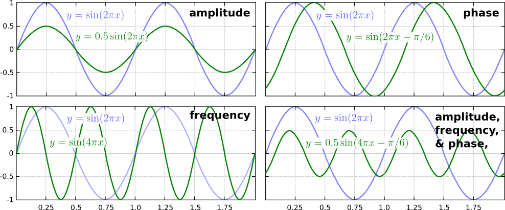
Wavelets measure displacement, or velocity, or acceleration (or some proxy for these things like voltage or capacitance), but eventually we can compute a signal that represents displacement. (In seismic reflection surveys, we don't care about the units.)

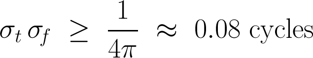
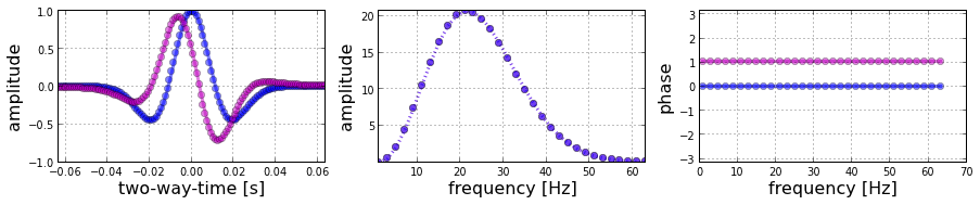
The Ricker wavelet represents an impulsive signal (the 'bang' of dynamite or the 'pop' of an airgun; let's leave Vibroseis out of it for now). The impulse is bandlimited ('band' as in radio band) — in other words, it doesn't contain all frequencies. Unfortunately, you need a lot of frequencies to represent very sudden or abrupt (short in time) things like bangs and pops, otherwise they spread out in time. Since our wavelet is restricted to a band of frequencies (eg 10 to 80 Hz), it must be (infinitely) spread out in time.

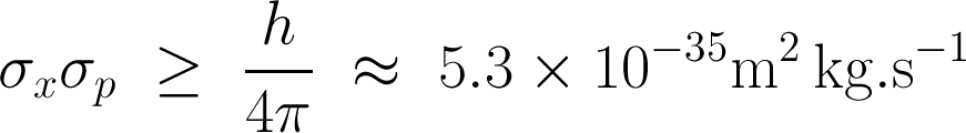
Additionally, since the frequencies don't contain what we call a 'DC' signal (0 Hz, in other words a bias or shift), it must return to zero when displaced. So it starts and ends on zero amplitude.

So the wavelet is spread out, and it starts and ends on zero amplitude. Why does it wiggle? In other words, why is seismic oscillatory? It's not the geophone: although it contains a spring (or something like one), its specially chosen/tuned to be able to move freely at the frequencies we're trying to record. So it's the stiffness of the earth itself which causes the oscillation, dissipating the vibrational energy (as heat) and damping the signal. At least, this explains why it dies out, but not really why it oscillates... Physics! Simple harmonic motion! Or something.

Yeah, I guess I’m a bit hazy on the micro-mechanics of wave propagation. Evan came to my rescue (see below), but I had a couple more things to say first:

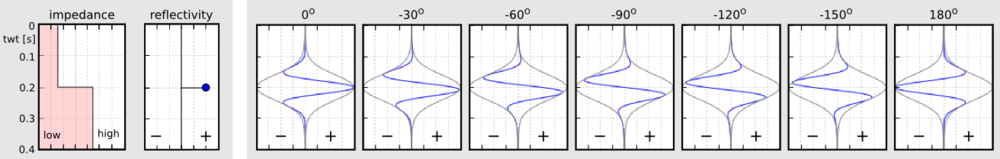
The other thing is that classic wavelets like the Ricker are noncausal, aka non-realizable, because they have energy at negative time (i.e. they are centered around t = 0) and there’s no such thing as negative time. This is a clue that a zero-phase wavelet is a geological convenience contrived during processing, not a physical thing. The field seismic data would contain a so-called 'minimum phase' wavelet, which looks more like what you'd expect a recording of a dynamite blast to look like (see below).

To try to make up for the fact that I trailed off at ‘simple harmonic motion’, Evan offered this:

If you imagine the medium being made up of a bunch of particles, then propagating a wave means causing a stress (say, sudden compression at the surface) and then stretching and squeezing those particles to accommodate that stress. A compression (which we may measure or draw as a peak) does not come without a stretching (a dilation or trough) of particles on either side. So a side lobe (or a dilation) has to exist in a way: the particles are connected together and stretch and squeeze when they feel pressure.

Choice of wavelet matters

There was more from Doug McClymont, who’s always up for some chat about wavelets. He pointed out that although high-bandwidth Ormsby wavelets have more sidelobes, they generally have lower amplitudes than a Ricker wavelet, whose sidelobes always have the same ampitude (exactly \( 2 \mathrm{e}^{-3/2} \)). He added:

I tend not to use Ricker wavelets for very much as you can't control the bandwidth of them (just the peak frequency) so they tend to be very narrow-band and have quite high (and constant) amplitude side lobes. As I work a lot with broadband seismic data I use Ormsby wavelets much more for any well-ties and seismic modelling.

Good reasons to use an Ormsby wavelet as your analaytic wavelet of choice! Check out this other post all about Ormsby wavelets and how to make them.

What do you think? Do you have an intuitive explanation for why wavelets have sidelobes? Ideally shorter than mine!

What is an Ormsby wavelet anyway?

If you dabble in reflection seismic analysis, you probably know the Ricker wavelet. We’ve visited it a few times on this blog — Evan once showed how to make and plot one, I looked at some analytic properties of it, and we even played golf with it.

The Ricker is everywhere, but it has an important limitation — bandwidth. Its shape in the frequency domain is roughly Gaussian (below, left), which is the reason it only really has one parameter: the central frequency. This kind of spectrum is sometimes okay for older seismic surveys, especially marine data, because it matches the bandwidth reasonably. But for modern surveys, or even old land data, we often want a broader set of frequencies — more of a trapezoidal spectral shape. We need the Ormsby wavelet:

ricker-vs-ormsby.png

How to make an Ormsby wavelet

The earliest reference I can find to the Ormsby wavelet is in an article by Harold Ryan entitled, Ricker, Ormsby, Klauder, Butterworth — a choice of wavelets, in the September 1994 issue of the CSEG Recorder. It’s not clear at all who Ormsby was, other than “an aeronautical engineer”. And I don’t think anyone outside exploration geophysics knows what an Ormsby is, they just call it a ‘bandpass filter’.

Ryan helpfully provided both a time-domain analytic expression — which turns out to have four typos use the classical definiton of the sinc function — and a plot:

The equation in Ryan, and my modified Figure 3 (right). the result of the equation is in red.

The equation in Ryan, and my modified Figure 3 (right). the result of the equation is in red.

ryan_ormsby-cf-expression-2.png

This equation does not produce the wavelet (black) in the plot, however, it produces the one I’ve added in red. If you find this surprising, you shouldn’t — in my experience, it’s very common for the words and/or maths in a paper not to match its figures. [Edit: as noted above, in this case it’s because of how NumPy’s sinc function is defined; see the comment from Robert Kern, below.] We established this at the SEG Repro Zoo in 2018. If an author is not required to produce code or data, it’s not very surprising; and even if they do, the peer review system is not set up for referees to do this kind of check — apart from anything else, it’s far too onerous. But I digress.

After some fiddling around, I realized that the expression being passed to NumPy’s sinc function should be \(ft\), not \(\pi ft\). This produces a result that matches the figure almost exactly (and, counting wiggles, has the right frequency). So here’s the result of that new expression, shown in green here with the original figure (black) and the same red wavelet as above:

ryan_ormsby-cf-bruges.png

This green thing is the wavelet implemented in bruges so it’s easy to produce it; the arguments are the duration (0.4 seconds), the sample interval dt (4 ms) and the corner frequencies f (5, 10, 40, and 45 Hz respectively):

bruges.filters.ormsby(duration=0.4, dt=0.004, f=[5, 10, 40, 45])

What about other examples from the literature?

Good question! Apart from my own Python code in bruges, I did find one or two other implementations:

So it seems from this tiny experiment that only one of the implementations I found matched the figure in the Ryan article perfectly. The other wavelets are variations on the theme. Which is probably fine — after all, they are all only models for real seismic impulses — but in the interests of scientific reproducibility, I think it underscores the importance of transparent methodology and publishing your code.


Update on 9 Feb: A conversation in Software Underground revealed that Petrel’s version of the Ormsby wavelet matches the bruges implementation — but with a triangular window multiplied in (similar to how a Hamming window is multiplied into the seismic.jl version.


518px-Jupyter_logo.svg.png

I pushed my Python Jupyter Notebook to the new repro-zoo repository on GitHub. Please feel free to fork this project and add your own attempted reproductions of computational geoscience papers.

The original repro-zoo repo from the 2018 event is on SEG’s GitHub.


References

Ryan, H (1994). Ricker, Ormsby, Klauder, Butterworth — a choice of wavelets. CSEG Recorder 19 (7). Available online.

Soo-Kyung Miong, Robert R. Stewart and Joe Wong (2007). Characterizing the near surface with VSP and well logs. CREWES Research Report 19. Available online.

It's Dynamic Range Day!

OK signal processing nerds, which side are you on in the Loudness War?

If you haven't heard of the Loudness War, you have some catching up to do! This little video by Matt Mayfield is kinda low-res but it's the shortest and best explanation I've been able to find. Watch it, then choose sides >>>>

There's a similar-but-slightly-different war going on in photography: high-dynamic-range or HDR photography is, according to some purists, an existential threat to photography. I'm not going to say any more about it today, but these HDR disasters speak volumes.

True amplitudes

The ideology at the heart of the Loudness War is that music production should be 'pure'. It's analogous to the notion that amplitudes in seismic images should be 'true', and just as nuanced. For some, the idea could be to get as close as possible to a live performance, for others it might be to create a completely synthetic auditory experience; for a record company the main point is to be noticed and then purchased (or at least searched for on Spotify). It reminds me a bit of the aesthetically

For a couple of decades, mainstream producers succumbed to the misconception that driving up the loudness — by increasing the mean amplitude, in turn by reducing the peaks and boosting the quiet passages — was the solution. But this seems to be changing. Through his tireless dedication to the cause, engineer Ian Shepherd has been a key figure in unpeeling this idée fixe. As part of his campaigning, he instituted Dynamic Range Day, and tomorrow is the 8th edition. 

If you want to hear examples of well-produced, dynamic music, check out the previous winners and runners up of the Dynamic Range Day Award — including tunes by Daft Punk, The XX, Kendrick Lamar, and at the risk of dating myself, Orbital.

The end is in sight

I'll warn you right now — this Loudness War thing is a bit of a YouTube rabbithole. But if you still haven't had enough, it's worth listening to the legendary Bob Katz talking about the weapons of war.

My takeaway: the war is not over, but battles are being won. For example, Spotify last year reduced its target output levels, encouraging producers to make more dynamic records. Katz ends his video with "2020 will be like 1980" — which is a good thing, in terms of audio engineering — and most people seem to think the Loudness War will be over.

R is for Resolution

Resolution is becoming a catch-all term for various aspects of the quality of a digital signal, whether it's a photograph, a sound recording, or a seismic volume.

I got thinking about this on seeing an ad in AAPG Explorer magazine, announcing an 'ultra-high-resolution' 3D in the Gulf of Mexico (right), aimed at site-survey and geohazard detection. There's a nice image of the 3D, but the only evidence offered for the 'ultra-high-res' claim is the sample interval in space and time (3 m × 6 m bins and 0.25 ms sampling). This is analogous to the obsession with megapixels in digital photography, but it is only one of several ways to look at resolution. The effect of increasing the sample interval of some digital images is shown in the second column here, compared to 200 × 200 pixels originals (click to zoom):

Another aspect of resolution is spatial bandwidth, which gets at resolving power, perhaps analogous to focus for a photographer. If the range of frequencies is too narrow, then broadband features like edges cannot be represented. We can simulate poor frequency content by bandpassing the data, for example smoothing it with a Gaussian filter (column 3).

Yet another way to think about resolution is precision (column 4). Indeed, when audiophiles talk about resolution, they are talking about bit depth. We usually record seismic with 32 bits per sample, which allows us to discriminate between a large number of values — but we often view seismic with only 6 or 8 bits of precision. In the examples here, we're looking at 2 bits. Fewer bits means we can't tell the difference between some values, especially as it usually results in clipping.

If it comes down to our ability to tell events (or objects, or values) apart, then another factor enters the fray: signal-to-noise ratio. Too much noise (column 5) impairs our ability to resolve detail and discriminate between things, and to measure the true value of, say, amplitude. So while we don't normally talk about the noise level as a resolution issue, it is one. And it may have the most variety: in seismic acquisition we suffer from thermal noise, line noise, wind and helicopters, coherent noise, and so on.

I can only think of one more impairment to the signals we collect, and it may be the most troubling: the total duration or extent of the observation (column 6). How much information can you afford to gather? Uncertainty resulting from a small window is the basis of the game Name That Tune. If the scale of observation is not appropriate to the scale we're interested in, we risk a kind of interpretation 'gap' — related to a concept we've touched on before — and it's why geologists' brains need to be helicoptery. A small 3D is harder to interpret than a large one. 

The final consideration is not a signal effect at all. It has to do with the nature of the target itself. Notice how tolerant the brick wall image is to the various impairments (especially if you know what it is), and how intolerant the photomicrograph is. In the astronomical image, the galaxy is tolerant; the stars are not. Notice too that trying to 'resolve' the galaxy (into a point, say) would be a mistake: it is inherently low-resolution. Indeed, its fuzziness is one of its salient features.

Have I missed anything? Are there other ways in which the recorded signal can suffer and targets can be confused or otherwise unresolved? How does illumination fit in here, or spectral bandwidth? What do you mean when you talk about resolution?


This post is an exceprt from my talk at SEG, which you can read about in this blog post. You can even listen to it if you're really bored. The images were generated by one of my IPython Notebooks that I point to in the talk, specifically images.ipynb

Astute readers with potent memories will have noticed that we have skipped Q in our A to Z. I just cannot seem to finish my post about Q, but I will!

The Safe Band ad is copyright of NCS SubSea. This low-res snippet qualifies as fair use for comment.

All the time freaks

SEG 2014Thursday was our last day at the SEG Annual Meeting. Evan and I took in the Recent developments in time-frequency analysis workshop, organized by Mirko van der Baan, Sergey Fomel, and Jean-Baptiste Tary (Vienna). The workshop came out of an excellent paper I reviewed this summer, which was published online a couple of weeks ago:

Tary, JB, RH Herrera, J Han, and M van der Baan (2014), Spectral estimation—What is new? What is next?, Rev. Geophys. 52. doi:10.1002/2014RG000461.

The paper compares the results of several time–frequency transforms on a suite of 'benchmark' signals. The idea of the workshop was to invite further investigation or other transforms. The organizers did a nice job of inviting contributors with diverse interests and backgrounds. The following people gave talks, several of them sharing their code (*):

  • John Castagna (Lumina) with a review of the applications of spectral decomposition for seismic analysis.
  • Steven Lin (NCU, Taiwan) on empirical methods and the Hilbert–Huang transform.
  • Hau-Tieng Wu (Toronto) on the application of transforms to monitoring respiratory patterns in animals.*
  • Marcílio Matos (SISMO) gave an entertaining, talk about various aspects of the problem.
  • Haizhou Yang (Standford) on synchrosqueezing transforms applied to problems in anatomy.*
  • Sergey Fomel (UT Austin) on Prony's method... and how things don't always work out.*
  • Me, talking about the fidelity of time–frequency transforms, and some 'unsolved problems' (for me).*
  • Mirko van der Baan (Alberta) on the results from the Tary et al. paper.

Some interesting discussion came up in the two or three unstructured parts of the session, organized as mini-panel discussions with groups of authors. Indeed, it felt like the session could have lasted longer, because I don't think we got very close to resolving anything. Some of the points I took away from the discussion:

  • My observation: there is no existing survey of the performance of spectral decomposition (or AVO) — these would be great risking tools.
  • Castagna's assertion: there is no model that predicts the low-frequency 'shadow' effect (confusingly it's a bright thing, not a shadow).
  • There is no agreement on whether the so-called 'Gabor limit' of time–frequency localization is a lower-bound on spectral decomposition. I will write more about this in the coming weeks.
  • Should we even be attempting to use reassignment, or other 'sharpening' tools, on broadband signals? To put it another way: does instantaneous frequency mean anything in seismic signals?
  • What statistical measures might help us understand the amount of reassignment, or the precision of time–frequency decompositions in general?

The fidelity of time–frequency transforms

My own talk was one of the hardest I've ever done, mainly because I don't think about these problems very often. I'm not much of a mathematician, so when I do think about them, I tend to have more questions than insights, so I made my talk into a series of questions for the audience. I'm not sure I got much closer to any answers, but I have a better idea of my questions now... which is a kind of progress I suppose.

Here's my talk (latest slidesGitHub repo). Comments and feedback are, as always, welcome.


The nonlinear ear

Hearing, audition, or audioception, is one of the Famous Five of our twenty or so senses. Indeed, it is the most powerful sense, having about 100 dB of dynamic range, compared to about 90 dB for vision. Like vision, hearing — which is to say, the ear–brain system — has a nonlinear response to stimuli. This means that increasing the stimulus by, say, 10%, does not necessarily increase the response by 10%. Instead, it depends on the power and bandwidth of the signal, and on the response of the system itself.

What difference does it make if hearing is nonlinear? Well, nonlinear perception produces some interesting effects. Some of them are especially interesting to us because hearing is analogous to the detection of seismic signals — which are just very low frequency sounds, after all.

Stochastic resonance (Zeng et al, 2000)

One of the most unintuitive properties of nonlinear detection systems is that, under some circumstances, most importantly in the presence of a detection threshold, adding noise increases the signal-to-noise ratio.

I'll just let you read that last sentence again.

Add noise to increase S:N? It might seem bizarre, and downright wrong, but it's actually a fairly simple idea. If a signal is below the detection threshold, then adding a small Goldilocks amount of noise can make the signal 'peep' above the threshold, allowing it to be detected. Like this:

I have long wondered what sort of nonlinear detection system in geophysics might benefit from a small amount of noise. It also occurs to me that signal reconstruction methods like compressive sensing might help estimate that 'hidden' signal from the few semi-random samples that peep above the threshold. If you know of experiments in this, I'd love to hear about it.

Better than Heisenberg (Oppenheim & Magnasco, 2012)

Denis Gabor realized in 1946 that Heisenberg's uncertainty principle also applies to linear measures of a signal's time and frequency. That is, methods like the short-time Fourier transform (STFT) cannot provide the time and the frequency of a signal with arbitrary precision. Mathematically, the product of the uncertainties has some minimum, sometimes called the Fourier limit of the time–bandwidth product.

So far so good. But it turns out our hearing doesn't work like this. It turns out we can do better — about ten times better.

Oppenheim & Magnasco (2012) asked subjects to discriminate the timing and pitch of short sound pulses, overlapping in time and/or frequency. Most people were able to localize the pulses, especially in time, better than the Fourier limit. Unsurprisingly, musicians were especially sensitive, improving on the STFT by a factor of about 10. While seismic signals are not anything like pure tones, it's clear that human hearing does better than one of our workhorse algorithms.

Isolating weak signals (Gomez et al, 2014)

One of the most remarkable characteristics of biological systems is adaptation. It seems likely that the time–frequency localization ability most of us have is a long-term adaption. But it turns out our hearing system can also rapidly adapt itself to tune in to specific types of sound.

Listening to a voice in a noisy crowd, or a particular instrument in an orchestra, is often surprisingly easy. A group at the University of Zurich has figured out part of how we do this. Surprisingly, it's not high-level processing in the auditory cortex. It's not in the brain at all; it's in the ear itself.

That hearing is an active process was known. But the team modeled the cochlea (right, purple) with a feature called Hopf bifurcation, which helps describe certain types of nonlinear oscillator. They established a mechanism for the way the inner ear's tiny mechanoreceptive hairs engage in active sensing.

What does all this mean for geophysics?

I have yet to hear of any biomimetic geophysical research, but it's hard to believe that there are no leads here for us. Are there applications for stochastic resonance in acquisition systems? We strive to make receivers with linear responses, but maybe we shouldn't! Could our hearing do a better job of time-frequency localization than any spectral decomposition scheme? Could turning seismic into music help us detect weak signals in the geological noise?

All very intriguing, but of course no detection system is perfect... you can fool your ears too!

References

Zeng FG, Fu Q, Morse R (2000). Human hearing enhanced by noise. Brain Research 869, 251–255.

Oppenheim, J, and M Magnasco (2013). Human time-frequency acuity beats the Fourier uncertainty principle. Physical Review Letters. DOI 10.1103/PhysRevLett.110.044301 and in the arXiv.

Gomez, F, V Saase, N Buchheim, and R Stoop (2014). How the ear tunes in to sounds: A physics approach. Physics Review Applied 1, 014003. DOI 10.1103/PhysRevApplied.1.014003.

The stochastic resonance figure is original, inspired by Simonotto et al (1997), Physical Review Letters 78 (6). The figure from Oppenheim & Magnasco is copyright of the authors. The ear image is licensed CC-BY by Bruce Blaus

What is the Gabor uncertainty principle?

This post is adapted from the introduction to my article Hall, M (2006), Resolution and uncertainty in spectral decomposition. First Break 24, December 2006. DOI: 10.3997/1365-2397.2006027. I'm planning to delve into this a bit, partly as a way to get up to speed on signal processing in Python. Stay tuned.


Spectral decomposition is a powerful way to get more from seismic reflection data, unweaving the seismic rainbow.There are lots of ways of doing it — short-time Fourier transform, S transform, wavelet transforms, and so on. If you hang around spectral decomposition bods, you'll hear frequent mention of the ‘resolution’ of the various techniques. Perhaps surprisingly, Heisenberg’s uncertainty principle is sometimes cited as a basis for one technique having better resolution than another. Cool! But... what on earth has quantum theory got to do with it?

A property of nature

Heisenberg’s uncertainty principle is a consequence of the classical Cauchy–Schwartz inequality and is one of the cornerstones of quantum theory. Here’s how he put it:

At the instant of time when the position is determined, that is, at the instant when the photon is scattered by the electron, the electron undergoes a discontinuous change in momen- tum. This change is the greater the smaller the wavelength of the light employed, i.e. the more exact the determination of the position. At the instant at which the position of the electron is known, its momentum therefore can be known only up to magnitudes which correspond to that discontinuous change; thus, the more precisely the position is determined, the less precisely the momentum is known, and conversely. — Heisenberg (1927), p 174-5.

The most important thing about the uncertainty principle is that, while it was originally expressed in terms of observation and measurement, it is not a consequence of any limitations of our measuring equipment or the mathematics we use to describe our results. The uncertainty principle does not limit what we can know, it describes the way things actually are: an electron does not possess arbitrarily precise position and momentum simultaneously. This troubling insight is the heart of the so-called Copenhagen Interpretation of quantum theory, which Einstein was so famously upset by (and wrong about).

Dennis Gabor (1946), inventor of the hologram, was the first to realize that the uncertainty principle applies to signals. Thanks to wave-particle duality, signals turn out to be exactly analogous to quantum systems. As a result, the exact time and frequency of a signal can never be known simultaneously: a signal cannot plot as a point on the time-frequency plane. Crucially, this uncertainty is a property of signals, not a limitation of mathematics.

Getting quantitative

You know we like the numbers. Heisenberg’s uncertainty principle is usually written in terms of the standard deviation of position σx, the standard deviation of momentum σp, and the Planck constant h:

In other words, the product of the uncertainties of position and momentum is small, but not zero. For signals, we don't need Planck’s constant to scale the relationship to quantum dimensions, but the form is the same. If the standard deviations of the time and frequency estimates are σt and σf respectively, then we can write Gabor’s uncertainty principle thus:

So the product of the standard deviations of time, in milliseconds, and frequency, in Hertz, must be at least 80 ms.Hz, or millicycles. (A millicycle is a sort of bicycle, but with 1000 wheels.)

The bottom line

Signals do not have arbitrarily precise time and frequency localization. It doesn’t matter how you compute a spectrum, if you want time information, you must pay for it with frequency information. Specifically, the product of time uncertainty and frequency uncertainty must be at least 1/4π. So how certain is your decomposition?

References

Heisenberg, W (1927). Über den anschaulichen Inhalt der quantentheoretischen Kinematik und Mechanik, Zeitschrift für Physik 43, 172–198. English translation: Quantum Theory and Measurement, J. Wheeler and H. Zurek (1983). Princeton University Press, Princeton.

Gabor, D (1946). Theory of communication. Journal of the Institute of Electrical Engineering 93, 429–457.

The image of Werner Heisenberg in 1927, at the age of 25, is public domain as far as I can tell. The low res image of First Break is fair use. The bird hologram is form a photograph licensed CC-BY by Flickr user Dominic Alves

Great geophysicists #10: Joseph Fourier

Joseph Fourier, the great mathematician, was born on 21 March 1768 in Auxerre, France, and died in Paris on 16 May 1830, aged 62. He's the reason I didn't get to study geophysics as an undergraduate: Fourier analysis was the first thing that I ever struggled with in mathematics.

Fourier was one of 12 children of a tailor, and had lost both parents by the age of 9. After studying under Lagrange at the École Normale Supérieure, Fourier taught at the École Polytechnique. At the age of 30, he was an invited scientist on Napoleon's Egyptian campaign, along with 55,000 other men, mostly soldiers:

Citizen, the executive directory having in the present circumstances a particular need of your talents and of your zeal has just disposed of you for the sake of public service. You should prepare yourself and be ready to depart at the first order.
Herivel, J (1975). Joseph Fourier: The Man and the Physicist, Oxford Univ. Press.

He stayed in Egypt for two years, helping found the modern era of Egyptology. He must have liked the weather because his next major work, and the one that made him famous, was Théorie analytique de la chaleur (1822), on the physics of heat. The topic was incidental though, because it was really his analytical methods that changed the world. His approach of decomposing arbitrary functions into trignometric series was novel and profoundly useful, and not just for solving the heat equation

Fourier as a geophysicist

Late last year, Evan wrote about the reason Fourier's work is so important in geophysical signal processing in Hooray for Fourier! He showed how we can decompose time-based signals like seismic traces into their frequency components. And I touched the topic in K is for Wavenumber (decomposing space) and The spectrum of the spectrum (decomposing frequency itself, which is even weirder than it sounds). But this GIF (below) is almost all you need to see both the simplicity and the utility of the Fourier transform. 

In this example, we start with something approaching a square wave (red), and let's assume it's in the time domain. This wave can be approximated by summing the series of sine waves shown in blue. The amplitudes of the sine waves required are the Fourier 'coefficients'. Notice that we needed lots of time samples to represent this signal smoothly, but require only 6 Fourier coefficients to carry the same information. Mathematicians call this a 'sparse' representation. Sparsity is a handy property because we can do clever things with sparse signals. For example, we can compress them (the basis of the JPEG scheme), or interpolate them (as in CGG's REVIVE processing). Hooray for Fourier indeed.

The watercolour caricature of Fourier is by Julien-Leopold Boilly from his work Album de 73 Portraits-Charge Aquarelle’s des Membres de I’Institute (1820); it is in the public domain.

Read more about Fourier on his Wikipedia page — and listen to this excellent mini-biography by Marcus de Sautoy. And check out Mostafa Naghizadeh's chapter in 52 Things You Should Know About Geophysics. Download the chapter for free!

P is for Phase

Seismic is about acoustic vibration. The archetypal oscillation, the sine wave, describes the displacement y of a point around a circle. You only need three pieces of information to describe it perfectly: the size of the circle, the speed at which it rotates around the circle, and where it starts from expressed as an angle. These quantities are better known as the amplitude, frequency, and phase respectively. These figures show how varying each of them affects the waveform:

So phase describes the starting point as an angle, but notice that this manifests itself as an apparent lateral shift in the waveform. For seismic data, this means a time shift. More on this later. 

What about seismic?

We know seismic signals are not so simple — they are not repetitive oscillations — so why do the words amplitudefrequency and phase show up so often? Aren't these words horribly inadequate?

Not exactly. Fourier's methods allow us to construct (and deconstruct) more complicated signals by adding up a series of sine waves, as long as we get the amplitude, frequency and phase values right for each one of them. The tricky part, and where much of where the confusion lies, is that even though you can place your finger on any point along a seismic trace and read off a value for amplitude, you can't do that for frequency or phase. The information for those are only unlocked through spectroscopy.

Phase shifts or time shifts?

The Ricker wavelet is popular because it can easily be written analytically, and it is comprised of a considerable number of sinusoids of varying amplitudes and frequencies. We might refer to a '20 Hz Ricker wavelet' but really it contains a range of frequencies. The blue curve shows the wavelet with phase = 0°, the purple curve shows the wavelet with a phase shift of π/3 = 60° (across all frequencies). Notice how the frequency content remains unchanged.

So for a seismic reflection event (below), phase takes on a new meaning. It expresses a time offset between the reflection and the maximum value on the waveform. When the amplitude maximum is centered at the reflecting point, it is equally shaped on either side — we call this zero phase. Notice how variations in the phase of the event alter the relative position of the peak and sidelobes. The maximum amplitude of the event at 90° is only about 80% of the amplitude at zero phase. This is why I like to plot traces along with their envelope (the grey lines). The envelope contains all possible phase rotations. Any event whose maximum value does not align with the maximum on the envelope is not zero phase.

Understanding the role of phase in time series analysis is crucial for both data processors aiming to create reliable data, and interpreters who operate under the assertion that subtle variations in waveform shape can be attributed to underlying geology. Waveform classification is a powerful attribute... but how reliable is it?

In a future post, I will cover the concept of instantaneous phase on maps and sections, and some other practical interpretation tips. If you have any of your own, share them in the comments.

Additional reading
Liner, C (2002). Phase, phase, phase. The Leading Edge 21, p 456–7. Abstract online.

Segmentation and decomposition

Day 4 of the SEG Annual Meeting in Las Vegas was a game of two halves: talks in the morning and workshops in the afternoon. I caught two signal processing talks, two image processing talks, and two automatic interpretation talks, then spent the afternoon in a new kind of workshop for students. My highlights:

Anne Solberg, DSB, University of Oslo

Evan and I have been thinking about image segmentation recently, so I'm drawn to those talks (remember Halpert on Day 2?). Angélique Berthelot et al. have been doing interesting work on salt body detection. Solberg (Berthelot's supervisor) showed some remarkable results. Their algorithm:

  1. Compute texture attributes, including Haralick and wavenumber textures (Solberg 2011)
  2. Supervised Bayesian classification (we've been using fuzzy c-means)
  3. 3D regularization and segmentation (okay, I got a bit lost at this point)

The results are excellent, echoing human interpretation well (right) — but having the advantage of being objective and repeatable. I was especially interested in the wavenumber textures, and think they'll help us in our geothermal work. 

Jiajun Han, BLISS, University of Alberta

The first talk of the day was that classic oil industry: a patented technique with an obscure relationship to theory. But Jiajun Han and Mirko van der Baan of the University of Alberta gave us the real deal — a special implementation of empirical mode decomposition, which is a way to analyse time scales (frequencies, essentially), without leaving the time domain. The result is a set of intrinsic mode functions (IMFs), a bit like Fourier components, from which Han extracts instantaneous frequency. It's a clever idea, and the results are impressive. Time–frequency displays usually show smearing in either the time or frequency domain, but Han's method pinpoints the signals precisely:

That's it from me for SEG — I fly home tomorrow. It's tempting to stay for the IQ Earth workshop tomorrow, but I miss my family, and I'm not sure I can crank out another post. If you were in Vegas and saw something amazing (at SEG I mean), please let us know in the comments below. If you weren't, I hope you've enjoyed these posts. Maybe we'll see you in Houston next year!

More posts from SEG 2012.

The images adapted from Berthelot and Han are from the 2012 Annual Meeting proceedings. They are copyright of SEG, and used here in accordance with their permissions guidelines.