The procedural generation of geology

Procedural generation is a way of faking stuff with computers. But by writing code, or otherwise defining algorithms — not by manually choosing or composing or sculpting things. It’s used to produce landscapes and other assets in computer games, or just to make beautiful things. Honestly, I know almost nothing about it, and I don’t play computer games, so I’m really just coming at it from the ‘beautiful things’ side. So let’s just stick to looking at some examples…

Robert Hodgin produces jaw-dropping images, and happily one of his favourite subjects is meandering rivers. Better yet, Harold Fisk’s maps are among his inspirations. The results are mindblowing — just check this animation out:

What’s really remarkable is that everything on that map is procedurally generated: the roadways, the vegetation, the wonderful names.

If you love meanders (who doesn’t love meanders?), then you also need to know about Zoltan Sylvester’s work (not to mention his Etsy store). He produces some great animations, and also maintains some open-source Python projects (e.g. meanderpy) for producing them, so you can get stuck in and make your own.

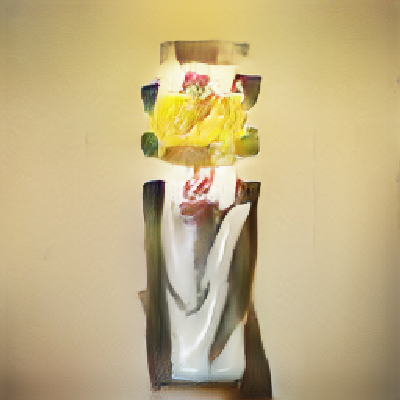
It’s not just about meanders. Artist Tyler Hobbs has produced some striking images that strongly resemble structural cross-sections. In this thread he mentions that this wasn’t his goal, they just came out that way.

Mattias Herder, a space-obsessed viz wizard, did intend to produce crystals though. He’s using Houdini software, which I believe is also what Robert Hodgin uses for his maps. I wonder if any geologists are using it…

Landscapes are one of the big areas of application of this sort of tech, and while not strictly geological, I love these frozen vistas by French artist Guillaume Cottet:

Finally, this example from digital artist Ian Smith hints at a bit of the creative process. This guy really knows how to make rocks…

This is all so much magic to me, but I’m intrigued. Like the black hole in Interstellar, could this kind of work actually shed light on how dynamic, non-linear natural systems work? Or is it just an illusion?

Does your machine learning smell?

Martin Fowler and Kent Beck popularized the term ‘code smell’ in the book Refactoring. They were describing the subtle signs of deeper trouble in code — signs that a program’s source code might need refactoring (restructuring and rewriting). There are too many aromas to list here, but here are some examples (remember, these things are not necessarily problems in themselves, but they suggest you need to look more closely):

  • Duplicated code.

  • Contrived complexity (also known as showing off).

  • Functions with many arguments, suggesting overwork.

  • Very long functions, which are hard to read.

More recently, data scientist Felienne Hermans applied the principle to the world’s number one programming environment: spreadsheets. The statistics on spreadsheet bugs are quite worrying, and Hermans enumerated the smells that might lead you to them. Here are four of her original five ‘formula’ smells, notice how they correspond to the code smells above:

  • Duplicated formulas.

  • Conditional complexity (e.g. nested IF statements).

  • Multiple references, analogous to the ‘many arguments’ smell.

  • Multiple operations in one cell.

What does a machine learning project smell like?

Most machine learning projects are code projects, so some familiar smells might be emanating from the codebase (if we even have access to it). But machine learning models are themselves functions — machines that map input X to some target y. And even if the statistical model is simple, like a KNN classifier, the workflow is a sort of ‘metamodel’ and can have complexities of its own. So what are the ‘ML smells’ that might alert us to deeper problems in our prediction tools?

I asked this question on Twitter (below) and in the Software Underground

I got some great responses. Here are some ideas adapted from them, with due credit to the people named:

  • Very high accuracy, especially a complex model on a novel task. (Ari Hartikainen, Helsinki and Lukas Mosser, Athens; both mentioned numbers around 0.99 but on earth science problems I start to get suspicious well before that: anything over 0.7 is excellent, and anything over 0.8 suggests ‘special efforts’ have been made.)

  • Excessive precision on hyperparameters might suggest over-tuning. (Chris Dinneen, Perth)

  • Counterintuitive model weights, e.g. known effects have low feature importance. (Reece Hopkins, Anchorage)

  • Unreproducible, non-deterministic code, e.g. not setting random seeds. (Reece Hopkins again)

  • No description of the train–val–test split, or justification for how it was done. Leakage between training and blind data is easy to introduce with random splits in spatially correlated data. (Justin Gosses, Houston)

  • No discussion of ground truth and how the target labels relate to it. (Justin Gosses again)

  • Less than 80% of the effort spent on preparing the data. (Michael Pyrcz, Austin — who actually said 90%)

  • No discussion of the evaluation metric, eg how it was selected or designed (Dan Buscombe, Flagstaff)

  • No consideration of the precision–recall trade-off, especially in a binary classification task. (Dan Buscombe again)

  • Strong class imbalance and no explicit mention of how it was handled. (Dan Buscombe again)

  • Skewed feature importance (on one or two features) might suggest feature leakage. (John Ramey, Austin)

  • Excuses, excuses — “we need more data”, “the labels are bad”, etc. (Hallgrim Ludvigsen, Stavanger)

  • AutoML, e.g. using a black box service, or an exhaustive automated seach of models and hyperparameters.

That’s already a long list, but I’m sure there are others. Or perhaps some of these are really the same thing, or are at least connected. What do you think? What red — or at least yellow — flags do you look out for when reviewing machine learning projects? Let us know in the comments below.


If you enjoyed this post, check out the Machine learning project review checklist I wrote bout last year. I’m currently working on a new version of the checklist that includes some tips for things to look for when going over the checklist. Stay tuned for that.


The thumbnail for this post was generated automatically from text (something like, “a robot smelling a flower”… but I made so many I can’t remember exactly!). Like a lot of unconstrained image generation by AI’s, it’s not great, but I quite like it all the same.

The AI is LXMERT from the Allen Institute. Try it out or read the paper.

download (7).png

x lines of Python: static basemaps with contextily

Difficulty rating: Beginner

Something that is often useful in planning is to have a basemap of the area in which you have data or an interest. This can be made using a number of different tools, up to and including full-fledged GIS software, but we will use Contextily for a quick static basemap using Python. Installation is as simple as using conda install contextily or pip install contextily.

The steps that we want to take are the following, expressed in plain English, each of which will roughly be one line of code:

  1. Get a source for our basemap (placenames and similar things)
  2. Get a source for our geological map
  3. Get the location that we would like to map
  4. Plot the location with our geological data
  5. Add the basemap to our geological map
  6. Add the attribution for both maps
  7. Plot our final map

We will start with the imports, which as usual do not count:

 
import contextily as ctx
import matplotlib.pyplot as plt

Contextily has a number of built-in providers of map tiles, which can be accessed using the ctx.providers dictionary. This is nested, with some providers offering multiple tiles. An example is the ctx.providers.OpenStreetMap.Mapnik provider, which contains the following:

 
{'url': 'https://{s}.tile.openstreetmap.org/{z}/{x}/{y}.png',
 'max_zoom': 19,
 'attribution': '(C) OpenStreetMap contributors',
 'name': 'OpenStreetMap.Mapnik'}

The most important parameter in the dictionary for each provider is the url. These are of the form example.com/{z}/{x}/{y}.png. The {z} is the zoom level, while {x} and {y} relate to the latitude and longitude of a given tile, respectively. Note that these are the same as those used by interactive Slippy maps; contextily just downloads them as a single static image.

The easiest is to use one of these providers, but we can also define our own provider, using the above pattern for the URL. For geological data, the Macrostrat project is a great resource, especially because they have a tileserver supplying some detail. Their tileserver can be added using

 
geology_tiles = 'https://tiles.macrostrat.org/carto/{z}/{x}/{y}.png'

We also need a place to map. Contextily has a geocoder that can return the tiles covering a given location. It uses OpenStreetMap, so anything that is present there is useable as a location. This includes countries (e.g. 'Paraguay'), provinces/states ('Nova Scotia'), cities ('Lubumbashi'), and so on.

We will use Nova Scotia as our area of interest, as well as giving our desired map tiles. We can also use .plot() on the Place object to get a look at it immediately, using that basemap.

 
ctx.Place('Nova Scotia', source=ctx.providers.CartoDB.Positron).plot()
The Positron style from Carto for Nova Scotia.

The Positron style from Carto for Nova Scotia.

We'll use a different basemap though:

 
basemap = ctx.providers.Stamen.Toner

We can create the Place with our desired source — geology_tiles in this case — and then plot this on the basemap with some transparency. We will also add an attribution, since we need to credit MacroStrat.

 
place = ctx.Place('Nova Scotia', source=geology_tiles)

base_ax = place.plot()
ctx.add_basemap(ax=base_ax, source=basemap, alpha=0.5)
text = basemap.attribution + ' | Geological data: MacroStrat.org (CC-BY)'
ctx.add_attribution(ax=base_ax, text=text)

Finally, after a plt.show() call, we get the following:

nova_scotia_geology.png

Obviously this is still missing some important things, like a proper legend, but as a quick overview of what we can expect in a given area, it is a good approach. This workflow is probably better suited for general location maps.

Contextily also plays well with geopandas, allowing for an easy locality map of a given GeoDataFrame. Check out the accompanying Notebook for an example.

Binder  Run the accompanying notebook in MyBinder

Geoscientist, challenge thyself

No costume is required for solving geocomputing kata

No costume is required for solving geocomputing kata

One of the highlights of my year is the Advent of Code, a sort of advent calendar for nerds. Its creator, Eric Wastl (hear his story), releases a new puzzle every day from the 1st of the month up to Christmas day. And the productivity of the global developer community goes down 74%.

Ever since the first one I tried, I’ve been wondering what geological coding challenges might look like. And now, 18 months later… well, I still don’t know, but I’ve made some anyway!

Puzzle number 1 (or 0)

Here’s how the first one starts:

You have a string of lithology codes, reading from the bottom up of a geological section. There is a sample every metre. There are three lithologies:

  • Mudstone
  • Fine sandstone or siltstone
  • Sandstone

The strings look like this:

    ...MFFSSFSSSS...

Your data, when you receive it, will be much longer than this.

We need to get some geological information from this string of codes. Specifically, you need to answer 3 questions:

  1. What is the total thickess in metres of sandstone (S)? Each sample represents one metre.
  2. How many sandstone beds are there? A bed is a contiguous group of one lithology, so MMFFF is 2 beds, one of M and one of F.
  3. How many times does the most common upwards bed transition occur? Do not include transitions from a lithology to itself.

You can download your own personal dataset, which in this case has 20,000 lithology codes. Then you can try to answer the questions, one at a time. You can use any programming language — indeed, any method at all — to solve the problems, you give an answer back to the server, and it will tell you if you are correct or not.

There are, as of right now, five ‘chapters’, covering topics from naming rock samples to combining map layers. You will receive the name of the next chapter when you correctly answer the final question of the three or four in each challenge.

If you’d like to give it a try, there’s a live starter Jupyter notebook here:

https://ageo.co/kata-live

Or, if you prefer, there’s a static notebook at https://ageo.co/kata, or you can dive directly into the web API for the first challenge: https://kata.geosci.ai/challenge/sequence

Do let us know how you get on!

Learn to code in 2020

Happy New Year! I hope 2020 is going well so far and that you have audacious plans for the new decade.

Perhaps among your plans is learning to code — or improving your skills, if you’re already on the way. As I wrote in 2011, programming is more than just writing code: it’s about learning a new way to think, not just about data but about problems. It’s also a great way to quickly raise your digital literacy — something most employers value more each year. And it’s fun.

We have three public courses planned for 2020. We’re also planning some public hackathons, which I’ll write about in the next week or three. Meanwhile, here’s the lowdown on the courses:

Lausanne in March

Rob Leckenby will be teaming up with Valentin Metraux of Geo2X to teach this 3-day class in Lausanne, Switzerland. We call it Intro to Geocomputing and it’s 100% suitable for beginners and people with less than a year or so of experience in Python. By the end, you’ll be able to read and write Python, write functions, read files, and run Jupyter Notebooks. More info here.

Amsterdam in June

If you can’t make it to Lausanne, we’ll be repeating the Intro to Geocomputing class in Amsterdam, right before the Software Underground’s Amstel Hack hackathon event (and then the EAGE meeting the following week). Check out the Software Underground Slack — look for the #amstel-hack-2020 channel — to find out more about the hackathon. More info here.

Houston in June

There’s also a chance to take the class in the US. The week before AAPG (which clashes with EAGE this year, which is very weird), we’ll be teaching not one but two classes: Intro to Geocomputing, and Intro to Machine Learning. You can take either one, or both — but be aware that the machine learning class assumes you know the basics of Python and NumPy. More info here.

In-house options

We still teach in-house courses (last year we taught 37 of them!). If you have more than about 5 people to train, then in-house is probably the way to go; we’d be delighted to work with you to figure out the best curriculum for your team.

Most of our classes fall into one of the following categories:

  • Beginner classes like the ones described above, usually 3 days.

  • Machine learning classes, like the Houston class above, usually 2 or 3 days.

  • Other more advanced classes built around engineering skills (object-oriented programming, testing, packaging, and so on), usually 3 days.

  • High-level digital literacy classes for middle to upper management, usually 1 day.

We also run hackathons and design sprints for teams that are trying to solve tricky problems in the digital subsurface, but those are another story…

Get in touch if you want more info about any of these.


Whatever you want to learn in 2020, give it everything you have. Schedule time for it. The discipline will pay off. If we can help or support you somehow, please let us know — above all, we want you to succeed.

Superpowers for striplogs

In between recent courses and hackathons, I’ve been chipping away at some new features in striplog. An open-source Python package, striplog handles irregularly sampled data, like lithologic intervals, chronostratigraphic zones, or anything that isn’t regularly sampled like, say, a well log. Instead of defining what is present at every depth location, you define intervals with a top and a base. The interval can contain whatever you like: names of rocks, images, or special core analyses, or anything at all.

You can read about all of the newer features in the changelog, but let’s look at a couple of the more interesting ones…

Binary morphology filters

Sometimes we’d like to simplify a striplog a bit, for example by ‘weeding out’ the thin beds. The tool has long had a method prune to systematically remove all intervals (e.g. beds) thinner than some cutoff; one can then optionally anneal the gaps, and merge the resulting striplog to combine similar neighbours. The result of this sequence of operations (prune, anneal, merge, or ‘PAM’) is shown below on the left.

striplog_binary_ops.png

If the intervals of a striplog have at least one property of a binary nature — with only two states, like sand and shale, or pay and non-pay — one can also use binary morphological operations. This well-known image processing technique aims to simplify data by eliminating small things. The result of opening vs closing operations is shown above.

Markov chains

I wrote about Markov chains earlier this year; they offer a way to identify bias in the order of units in a stratigraphic column. I’ve now put all the code into striplog — albeit not in a very fancy way. You can import the Markov_chain class from striplog.markov, then use it in exactly the same way as in the notebook I shared in that Markov chain post:

I started with some pseudorandom data (top) representing a known succession of Mudstone (M), Siltstone (S), Fine Sandstone (F) and coarse sandstone (C). Then I generate a Markov chain model of the succession. The chi-squared test indicates that the succession is highly unlikely to be unordered. We can look at the normalized difference matrix, generate a synthetic sequence of lithologies, or plot the difference matrix as a heatmap or a directed graph. The graph illustrates the order we originally imposed: M-S-F-C.

There is one additional feature compared to the original implementation: multi-step Markov chains. Previously, I was only looking at immediately adjacent intervals (beds or whatever). Now you can look at actual vs expected transition frequencies for next-but-one interval, or next-but-two. Don’t ask me how to interpret that information though…

Other new things

  • New ways to anneal. Now the user can choose whether the gaps in the log are filled in by flooding upwards (that is, by extending the interval below the gap upwards), flooding downwards (extending the upper interval), or flooding symmetrically into the middle from both above and below, meeting in the middle. (Note, you can also fill gaps with another component, using the fill() method.)

  • New merging strategies. Now you can merge overlapping intervals by precedence, rather than by blending the contents of the intervals. Precedence is defined however you like; for example, you can choose to keep the thickest interval in all overlaps, or if intervals have a date, you could keep the latest interval.

  • Improved bar charts. The histogram is easier to use, and there is a new bar chart summary of intervals. The bars can be sorted by any property you like.

Try it out and help add new stuff

You can install the latest version of striplog using pip. It’s as easy as:

pip install striplog

Start by checking out the tutorial notebooks in the repo, especially Striplog_basics.ipynb. Let me know how you get on, or jump on the Software Underground Slack to ask for help.

Here are some things I’d like striplog to support in the future:

  • Stratigraphic prediction.

  • Well-to-well correlation.

  • More interactions with well logs.

What ideas do you have? Or maybe you can help define how these things should work? Either way, do get in touch or check out the Striplog repository on GitHub.

x lines of Python: Loading images

Difficulty rating: Beginner

We'd often like to load images into Python. Once loaded, we might want to treat them as images, for example cropping them, saving in another format, or adjusting brightness and contrast. Or we might want to treat a greyscale image as a two-dimensional NumPy array, perhaps so that we can apply a custom filter, or because the image is actually seismic data.

This image-or-array duality is entirely semantic — there is really no difference between images and arrays. An image is a regular array of numbers, or, in the case of multi-channel rasters like full-colour images, a regular array of several numbers: one for each channel. So each pixel location in an RGB image contains 3 numbers:

raster_with_RGB_triples.png

In general, you can go one of two ways with images:

  1. Load the image using a library that 'knows about' (i.e. uses language related to) images. The preeminent tool here is pillow (which is a fork of the grandparent of all Python imaging solutions, PIL).
  2. Load the image using a library that knows about arrays, like matplotlib or scipy. These wrap PIL, making it a bit easier to use, but potentially losing some options on the way.

The Jupyter Notebook accompanying this post shows you how to do both of these things. I recommend learning to use some of PIL's power, but knowing about the easier options too.

Here's the way I generally load an image:

 
from PIL import Image
im = Image.open("my_image.png")

(One strange thing about pillow is that, while you install it with pip install pillow, you still actually import and use PIL in your code.) This im is an instance of PIL's Image class, which is a data structure especially for images. It has some handy methods, like im.crop(), im.rotate(), im.resize(), im.filter(), im.quantize(), and lots more. Doing some of these operations with NumPy arrays is fiddly — hence PIL's popularity.

But if you just want your image as a NumPy array:

 
import numpy as np
arr = np.array(im)

Note that arr is a 3-dimensional array, the dimensions being row, column, channel. You can go off with arr and do whatever you need, then cast back to an Image with Image.fromarray(arr).

All this stuff is demonstrated in the Notebook accompanying this post, or you can use one of these links to run it right now in your browser:

Binder   Run the accompanying notebook in MyBinder


x lines of Python: Physical units

Difficulty rating: Intermediate

Have you ever wished you could carry units around with your quantities — and have the computer figure out the best units and multipliers to use?

pint is a nice, compact library for doing just this, handling all your dimensional analysis needs. It can also detect units from strings. We can define our own units, it knows about multipliers (kilo, mega, etc), and it even works with numpy and pandas.

To use it in its typical mode, we import the library then instantiate a UnitRegistry object. The registry contains lots of physical units:

 
import pint
units = pint.UnitRegistry()
thickness = 68 * units.m

Now thickness is a Quantity object with the value <Quantity(68, 'meter')>, but in Jupyter we see a nice 68 meter (as far as I know, you're stuck with US spelling).

Let's make another quantity and multiply the two:

 
area = 60 * units.km**2
volume = thickness * area

This results in volume having the value <Quantity(4080, 'kilometer ** 2 * meter')>, which pint can convert to any units you like, as long as they are compatible:

 
>>> volume.to('pint')
8622575788969.967 pint

More conveniently still, you can ask for 'compact' units. For example, volume.to_compact('pint') returns 8.622575788969966 terapint. (I guess that's why we don't use pints for field volumes!)

There are lots and lots of other things you can do with pint; some of them — dealing with specialist units, NumPy arrays, and Pandas dataframes — are demonstrated in the Notebook accompanying this post. You can use one of these links to run this right now in your browser if you like:

Binder   Run the accompanying notebook in MyBinder

Open In Colab   Run the notebook in Google Colaboratory (note the install cell at the beginning)

That's it for pint. I hope you enjoy using it in your scientific computing projects. If you have your own tips for handling units in Python, let us know in the comments!


There are some other options for handling units in Python:

  • quantities, which handles uncertainties without also needing the uncertainties package.
  • astropy.units, part of the large astropy project, is popular among physicists.

The hack returns to Norway

Last autumn Agile helped Peter Bormann (ConocoPhillips Norge) and the FORCE consortium host the first geo-flavoured hackathon in Norway. Maybe you were there, or maybe you read about the nine fascinating machine learning projects here on the blog. If so, you’ll know it was a great event, so we’re doing it again!

Hackthon: 18 and 19 September
Symposium: 20 September


Check out last year’s projects here. Projects included Biostrat!, Virtual Metering, sketch2seis, and AVO ML — a really interesting AVO approach exploiting latent spaces (see image, right). Most of them are on GitHub and could be extended this year.

Part of what I love about these things is that we have no idea what the projects will be. As last year, there’ll be a pre-hackathon meetup in Storhaug the evening before Day 1 (on 17 September) — we’ll figure it all out there. In the meantime, if you have an idea check out the link at the end of this post where you can share and discuss it with others.


20180919_FUJ8654.jpg

The hackathon will be followed by a one-day symposium on machine learning in the subsurface (left). This well attended event was also excellent last year, and promises to deliver again in 2019. Peter did a briliant job of keeping things rooted in real results from real research, so you won’t be subjected to the parade of marketing talks you might have been subjected to at certain other conferences.


Find out more and sign up on NPD.no! Don’t delay; places are limited.

Submit and discuss project ideas on Agile’s Events page. Note that this does not sign you up for the event.

Get on softwareunderground.com/slack to discuss the event in the #force-hack-2019 channel.

See you there!

Is your data digital or just pseudodigital?

pseudodigital_analog.png

A rite of passage for a geologist is the making of an original geological map, starting from scratch. In the UK, this is known as the ‘independent mapping project’ and is usually done at the end of the second year of an undergrad degree. I did mine on the eastern shore of the Embalse de Santa Ana, just north of Alfarras in Catalunya, Spain. (I wrote all about it back in 2012.)

The map I drew was about as analog as you can get. I drew it with Rotring Rapidograph pens on drafting film. Mistakes had to be painstakingly scraped away with a razor blade. Colour had to be added in pencil after the map had been transferred onto paper. There is only one map in existence. The data is gone. It is absolutely unreproducible.

pseudodigital_palaeo.png

Digitize!

In order to show you the map, I had to digitize it. This word makes it sound like the map is now ‘digital data’, but it’s really not useful for anything scientific. In other words, while it is ‘digital’ in the loosest sense — it’s a bunch of binary bits in the cloud — it is not digital in the sense of organized data elements with semantic meaning. Let’s call this non-useful format palaeodigital. The lowest rung on the digital ladder.

You can get palaeodigital files from many state and national data repositories. For example, it’s how the Government of Nova Scotia stores its offshore seismic ‘data’ files — as TIFF files representing scans of paper sections submitted by operators. Wiggle trace, obviously, making them almost completely useless.

pseudodigital_proto.png

Protodigital

Nobody draws map by hand anymore, that would be crazy. Adobe Illustrator and (better) Inkscape mean we can produce beautifully rendered maps with about the same amount of effort as the hand-drawn version. But… this still isn’t digital. This is nothing more than a computerized rip-off of the analog workflow. The result is almost as static and difficult to edit as it was on film. (Wish you’d used a thicker line for your fault traces on those 20 maps? Have fun editing those files!)

Let’s call the computerization of analog workflows or artifacts protodigital. I’m thinking of Word and Powerpoint. Email. SeisWorks. Techlog. We can think of data in the same way… LAS files are really just a text-file manifestation of a composite log (plus their headers are often garbage). SEG-Y is nothing more than a bunch of traces with a sidelabel.


Together, palaeodigital and protodigital data might be called pseudodigital. They look digital, but they’re not quite there.

(Just to be clear, I made all these words up. They are definitely silly… but the point is that there’s a lot of room between analog and useful, machine-learning-ready digital.)


pseudodigital_digital.png

Digital data

So what’s at the top of the digital ladder? In the case of maps, it’s shapefiles or, better yet, GeoJSON. In these files, objects are described in terms of real geographic parameters, such at latitiude and longitude. The file contains the CRS (you know you need that, right?) and other things you might need like units, data provenance, attributes, and so on.

What makes these things truly digital? I think the following things are important:

  • They can all be self-documenting

  • …and can carry more or less arbitrary amounts of metadata.

  • They depend on open formats, some text and some binary, that are widely used.

  • There is free, open-source tooling for reading and writing these formats, usually with reference implementations in major languages (e.g. C/C++, Python, Java).

  • They are composable. Without too much trouble, you could write a script to process batches of these files, adapting to their content and context.

Here’s how non-digital versions of a document, e.g. a scholoarly article, compare to digital data:

pseudodigital_document.png

And pseudodigital well logs:

pseudodigital_log.png

Some more examples:

  • Photographs with EXIF data and geolocation.

  • GIS tools like QGIS let us make beautiful maps with data.

  • Drawing striplogs with a data-driven tool like Python striplog.

  • A fully-labeled HDF5 file containing QC’d, machine-learning-ready well logs.

  • Structured, metadata-rich documents, perhaps in JSON format.

Watch out for pseudodigital

Why does all this matter? It matters because we need digital data before we can do any analysis, or any machine learning. If you give me pseudodigital data for a project, I’m going to spend at least 50% of my time, probably more, making it digital before I can even get started. So before embarking on a machine learning project, you really, really need to know what you’re dealing with: digital or just pseudodigital?