This page is a high-level overview of our material. It will give you a flavour of the sort of data we use and the exercises we set. We do not teach the entire curriculum in one go. As a rough guide, we have about 2 days of content for each module. We love developing new components if there's something you don't see.
MODULE 0: Principles of geocomputing
We don't actually teach this module, but it drives everything we do.
- Everything is implemented in code: figures, charts, examples, etc.
- Everything is reproducible.
- Everything is in version control.
- Data must be digital and carry metadata.
- Important workflows belong in code.
MODULE 1: Getting started in Python
In this module we will get used to Python's syntax and explore some of its built-in functions. At the end, we will have a good overview of the basic toolset used by earth scientists everywhere, and be ready to dive deeper.
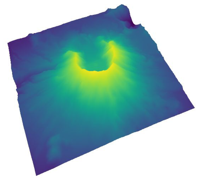
Manipulating and visualizing data
- Follow-along exercise: Make a topography map in 5 lines of code (right).
- Follow-along exercise: A lightweight 3D seismic visualization.
Variables and assignment
- Introduction to Python command line.
- Basic assignment syntax and dynamic typing.
- Asking for help. Finding help online.
Native data types
- int and float (and complex); why so many kinds of numbers?
- str.
- Type casting.
- String methods, strings as collections. Indexing and slicing.
- String formatting anf f-strings.
- Exercise: text processing practice manipulating formation names.
Operators and expressions
- Mathematical operations, comparison operators, booleans.
- Augmented assignment, multiple assignment.
- Copies and pointers.
- Exercise: some gentle rock physics.
Data collections and data structures
- list — indexing again, slicing again, striding, nested lists.
- Exercise: Getting ages from the geologic timescale. Practice indexing.
- tuple and set
- dict — mappings of key:value pairs.
- Exercise: Stratigraphic column: storing, retrieving and modifying entries in dicts.
- Exercise: Introduction to visualizing well logs: line plots vs scatter plots.
Flow control
- Iteration and iterables: for and while.
- Exercise: compute impedance and reflectivity in a well.
- List comprehensions.
- Exercise: convert for loops into list comprehensions.
- Making decisions: if-elif-else statements.
- Exercise: create a pay flag on a gamma-ray log.
Getting data, part 1
- Reading and writing text files.
- Exercise: create a dictionary of well tops from a ‘broken’ input text file.
- Functions
- Built-in functions, and importing modules.
- The anatomy of a function. Syntax, docstrings.
- Exercise: write a function that computes an impedance log.
- Exercise: write a function that computes reflection coefficients.
- Exercise: write a function that computes formation thicknesses.
- Sharing code via modules, importing and using modules.
- Exercise: Getting data from a sidewall core analysis report (csv file).
- Exercise: Get geological ages by processing pages.
- The Python standard library.
- External Python packages and PyPi.
MODULE 2: Scientific computing
In this module we will jump into numerical computing with NumPy. We'll also find out how to make charts in matplotlib, and discover the rich toolkits in the SciPy family. After Day 2, students will have some understanding of how to make useful scientific tools.
NumPy

- What is NumPy for? n-dimensional arrays!
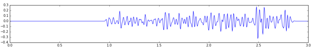
- A simple synthetic seismogram.
- Exercise: make a 2D wedge model.
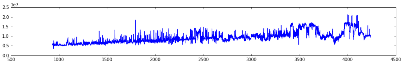
- Load and inspect a 1D wireline log.
- Exercise: compare list iteration to vectorized math to compute reflectivity.
- Load and inspect a 2D seismic section from Numpy binary.
- Exercise: plotting raster data with imshow.
- Load and inspect a 3D seismic volume from Numpy binary.
- Indexing into the cube, computing trace statistics.
- Visualize traces, sections, and timeslices.
- Exercise: load and visualize a seismic horizon.
matplotlib
- What is matplotlib?
- Exercise: Exploring plots.
- Seaborn, Plotly, Bokeh, and other plotting environments.
SciPy
- What's in the SciPy package?
- Interpolation: time conversion of a sonic log.
- Convolution.
- Exercise: make a simple synthetic seismogram.
- Complex seismic trace attributes — phase and envelope.
- Exercise: make an offset synthetic seismogram.
- Spectral analysis with scipy.
- Exercise: make a time-frequency plot of our synthetic.
Scikit-image and PIL
- What is image processing? What are scikit-image and PIL?
- Exercise: resize and recolour an image in PIL.
- Image segmentation.
- Exercise: find grains in a photomicrograph with scikit-image.
Pandas, a quick introduction
- What is pandas? When do we use pandas vs ndarrays?
- Exercise: Loading and cleaning a dataset with pandas.
- Exercise: A quick introduction to GeoPandas.
Reading and writing data files
- Persisting ndarrays, dataframes, and other objects. Pickling.
- Reading SEG-Y files with ObsPy. Writing SEG-Y files.
- Reading LAS files with lasio and welly. Writing LAS files.
- Reading and writing SHP files with fiona.
Getting data, part 2
- Databases. SQL vs NoSQL. Libraries for hitting databases.
- Exercise: Storing objects in a database, and retrieving them again. Querying.
- Exercise: Storing the same objects in a NoSQL database, msiemens's TinyDB.
MODULE 3: Practical programming
In this module, we look at some of the tools of the scientific programmer. You will come across most of them as soon as you start coding, and it can be a long and confusing path to figure out what they all are. We'll get you started with some basic concepts.
Writing code
- Text editors, IDES, Jupyter.
- Linting and PEP8.
- Documentation, testing, continuous integration.
Classes and object-oriented programming
- Everything is an object.
- Why use classes?
- Exercise: define a well log class with attributes and methods.
Version control
- Introduction to git and GitHub.
- Exercise: clone a project that interests you, and use it.
- Exercise: start a new repo for our well log class and get it set up.
Runtime
- Conda environments. Other options.
- Exercise: build and clone a conda environment for your project.
- Containers, Docker, and developer operations.
Test driven development
- Untested code is broken code.
- Writing tests.
- Exercise: write the first tests for our well log class.
Documentation
- Writing self-documenting code: docstrings and comments.
- Supporting documents and notebooks.
- Exercise: document our well log class.
Packaging
- Functions, files, modules, and packages — review.
- Setup.py, requirements.txt, PyPi, and everything else.
- Managing branches in git.
Getting better
- Tips for becoming a better programmer.
- Online resources. Conferences and meetings.
MODULE 4: Applications
We start to bring things together with a look at delivering useful tools to earth scientists, and other developers. We'll build a simple command-line application, we'll talk about GUIs, and then jump into the cloud — and web applications.
Command line tools
- Running Python programs: review.
- Getting arguments from the command line.
- Exercise: build a small tool to plot an LAS file.
Web applications
- Why you shouldn't build desktop applications.
- The web as an application: APIs, microservices.
- Protocols, standards, and patterns. REST.
- Useful packages: requests, flask.
- Exercise: Use a web-based service via its API: curvenam.es.
- An introduction to web applications with flask.
- Exercise: build and deploy a web service to make LAS plots.
Front end
- Front-end 'programming': HTML5, CSS, JavaScript.
- Exercise: add a simple front end to our app.
MODULE 5: Machine learning for geoscientists
Introduction
- Recognizing tasks suitable for machine learning.
- What's the difference between supervised and unsupervised learning?
- Recognizing regression vs classification tasks.
Data management for machine learning
- DataFrames: A new way to look at well logs.
- Exercise: loading a pandas DataFrame from a CSV.
- Exercise: building a pandas DataFrame from a LAS file.
- DataFrames vs arrays (vs Hadoop, Dask, etc).
The machine learning iterative loop
- Data — Getting the data. Loading and storing in an array and/or DataFrame
- Processing — data exploration, inspection, cleaning, and feature engineering.
- Model — What is a model? Training a Scikit-Learn model (for now).
- Results — assessing quality and performance metrics (accuracy, recall, F1,
- confusion matrices)
- Repeat — What can we do to improve performance?
- Exercise: predicting a missing well log.
- Exercise: improving the pay flag prediction.
- Exercise: Hugoton lithology prediction contest.
 Except where noted, this content is licensed